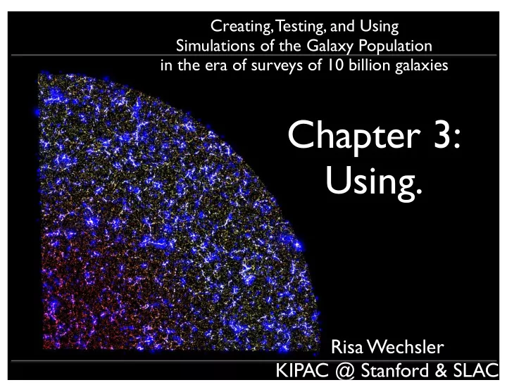

Creating, Testing, and Using Simulations of the Galaxy Population in the era of surveys of 10 billion galaxies Chapter 3: Using. Risa Wechsler KIPAC @ Stanford & SLAC
large cosmological simulations allow you to do many analyses in new ways
Inference from the Prior PDF of Cosmological Simulations.
basic idea: • let’s say you have an object (or objects) that you observe. • you know some of its observed properties. • you have a cosmological simulation that you think reproduces those properties well. • your simulation has a lot of volume, so that you would statistically expect to find many objects with these observed properties.
basic idea: continued • (for simplicity, consider the case where the cosmological model in your simulation is identical to the true cosmological model of our universe) • Catalogs from this cosmological simulation can be thought of as the prior PDF on the properties of your object. • You then importance sample this prior PDF with your observable data, to get the posterior PDF of some underlying property of the object in question.
example What is the mass of the Milky Way? Busha, Marshall et al (2011); Marshall, Busha, RW 2012 in prep
What observable information might tell us about this? • the rotation curve, as traced by stellar halo stars • the properties of the MW satellites: positions, masses, proper motions • motion with respect to Andromeda • etc...
• Large cosmological simulations contain millions of dark matter halos • We know the position mass, velocity, motions, internal properties of each one at every output time, plus their assembly histories • A halo catalog can be thought of as a set of samples drawn from our prior probability density function for galaxy halos
Bolshoi vs SDSS • Reproduces small and large scale clustering of galaxies • 100,000 halos have at least one sub-halo
• The Milky Way has two large satellite galaxies, the LMC and SMC
What can the existence and properties of these galaxies teach us about the properties and history of the MW?
Observational Constraints on the Milky Way – Not a “satellite” of a larger structure – Has exactly two satellites with v max > 50 km/s – No other substructures within 300 kpc with v max > 25km/s Sagittarius is next brightest with v max ~ 20 km/s (Strigari et al 10) LMC SMC v max ~65 km/s ~60 km/s Watkins, Evans, & An 2010; Kallivayalil, van der Marel, & Alcock r 0 50 kpc 60 kpc 06; Krachentsev et al 04; v rad 89 ± 4 km/s 23 ± 7 km/s van der Marel et al 02 Speed 378 ± 18 km/s 301 ± 52 km/s
What people often do: • very difficult measurement (e.g. proper motion of the MCs: observing the motion of stars relative to background quasars over a baseline of several years) • interpret in the context of simplified dynamical models • better: model the dynamics of halos in their true cosmological context; dynamics generated by an LCDM universe
• The Milky Way has exactly two satellite galaxies with v max > 50 km/s, the LMC and SMC • 36000 halos in Bolshoi have exactly two satellite galaxies with v max > 50 km/s.
Constrained halo catalogs • We have some intrinsic halo properties {x} e.g. mass, concentration, assembly history... • We have some data [d] for these objects. • What is the posterior for these intrinsic properties, given the data? • P({x}¦[d]) ̃ P ([d]¦{x})P({x})
Constrained halo catalogs • Subhalos in Bolshoi catalog Prior PDF: P 1 ( {M host ,r 1 ,v 1 ,r 2 ,v 2 ,...} ¦ H ) • Observations of Magellanic Clouds: Likelihood P 2 ( [r 1,obs ,v 1obs ,r 2,obs ,v 2,obs ] ¦ {x}, H) • New measurements: Posterior PDF P 3 ( {x} ¦ [d], H ) P 1 x P 2
Constrained halo catalogs • Posterior PDF P 3 ( {x} ¦ [d], H ) P 1 x P 2 • We want samples from P3, but we only have Importance ! Sampling samples from P1. Look at integrals: <x> = \int x P 3 dx = \int x (P 3 /P 1 ) P 1 dx = \int x P 2 P 1 dx ̃ \sum{ x P 2 } • Inferences are sums over prior samples, weighted by the likelihood
one of the “MW-like” halos
Weighing the Milky Way
How unusual is the MW halo? • Around 1 in 20 Milky Way- like galaxies have two Magellanic clouds (Busha et al 2011b) • The Magellanic Clouds are surprisingly close, and are moving surprisingly fast! What else can we learn?
When did the Magellanic Clouds arrive? • 72% chance they arrived within the last billion years, • and 50% chance they arrived together see also Boylan-Kolchin, Besla & Hernquist 2010
When did the Magellanic Clouds arrive? Visualization: Ralf Kaehler see Sky & Telescope cover, October 2012!
Importance sampling failure modes Additional uncertainty from N eff = 10 4 sampling noise 1. The parameter space is not well-sampled Large volumes are needed: we can then assert that we are studying the MW in its cosmological context (Copernicus, cf SDSS, etc) / larger volumes for rarer objects! 2. The importance weighting leaves too few samples, that then dominate the posterior 400 samples lie within 2- volume, but N eff = 10 4 Sampling noise is included in the statistical error bars, estimated by bootstrap resampling
Many possible applications • In this case: – apply more/tighter priors (e.g. new measurements of the LMC proper motions!) – look at the posterior distribution of other intrinsic properties, and learn more about the MW (e.g. satellite population, distribution and speeds of dark matter particles, etc.) • Many other interesting examples!
Weighing galaxies with halo catalogs • Can we measure the Local Group mass and history in the same way? Consuelo: ~100x Bolshoi volume
Preliminary results on the Local Group Isolated groups of 3 halos, Local group masses with M31 and M33 distance are dominated by M31 and radial velocity likelihoods (around 3 times M33 exists heavier than MW): +M31 kinematics M M31 formal uncertainty +M33 kinematics around 50% +MW mass M M33 log M200 estimates: MW: 12.0 +/- 0.1 prior M31: 12.66 +/- 0.15 M33: 11.7 +/- 0.3 M LG LG: 12.8 +/- 0.1 (errors are correlated) M MW M M31 M M33 M LG
The Timing Argument Isolated groups of 3 halos, with M31’s radial orbit Big Bang M31 and M33 distance and suggests a simple toy radial velocity likelihoods 0 Gyr model for the Local Group collapse M33 exists +M31 kinematics (Kahn & Woltjer 1959) M TA +M33 kinematics r = a (1 - cos ) +MW mass We can calibrate this by t = (a 3 /GM) 1/2 ( - sin ) computing M TA for each v = (GM/a) 1/2 sin / (1 - cos ) LG analog: A 200 M 200 = M TA / A 200 13.7 Gyr log A 200 estimates: v rad r, v, t Prior: -0.10 +/- 0.23 Posterior: -0.06 +/- 0.10 time M LG M TA A 200 v rad Li & White: 0.0+/-0.4
Weighing galaxies with halo catalogs • Can we measure the Local Group mass and history in the same way? Consuelo: ~100x Bolshoi volume • What is the shape of the Milky Way halo? What “missing satellite” population do we predict? • What is the distribution of dark matter in the Milky Way? • How could we include more satellites? When will importance sampling break down? How can we sample PDFs in (100 epochs x 100 parameters*) = 10000D? Importance sampling is very inefficient (need large volumes), but constrained realizations are expensive... Middle ground? * e.g. 2 mass profile params, 6D phase space, 3 angular momentum vector, 6 inertia tensor = 17 per halo x 5-6 halos ~ 100
Many possible applications • Velocities of galaxies in clusters? And in the large scale structure? • Motions of massive clusters (e.g. Bullet cluster) • Anything else where you have observations that relate to properties well predicted in simulations, and some intrinsic property you are interested in!
large cosmological simulations allow you to do many analyses in new ways
large cosmological simulations allow you to do many analyses in new ways... but care must be taken to properly estimate the impact of uncertainties
Example in galaxy cluster cosmology • two key steps in cluster cosmology: – find the clusters – weigh the clusters • cosmological analysis: – depends on relating these observed objects to predictions of the mass function of halos in a given cosmological model
Recommend
More recommend