Chapter 3 Parametric Models and Methods Models: Weibull ( includes - PDF document

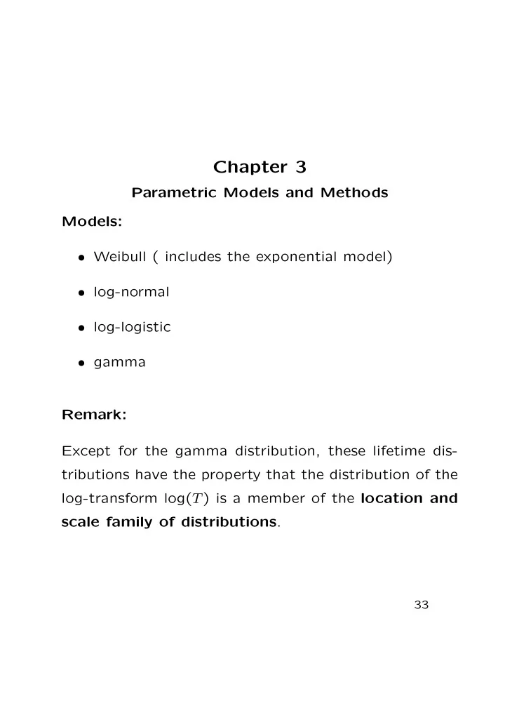
Chapter 3 Parametric Models and Methods Models: • Weibull ( includes the exponential model) • log-normal • log-logistic • gamma Remark: Except for the gamma distribution, these lifetime dis- tributions have the property that the distribution of the log-transform log( T ) is a member of the location and scale family of distributions . 33

Summary: The common features are: • The time T distributions have two parameters − scale = λ > 0 and shape = α > 0 . • In log-time, Y = log( T ), the distributions have two parameters − scale = σ = 1 location = µ = − log( λ ) and α . • Each can be expressed in the form Y = log( T ) = µ + σZ , where Z is the standard member; that is, µ = 0 ( λ = 1) and σ = 1 ( α = 1) . • They are log-linear models. The three distributions are summarized as follows: T ⇐ ⇒ Y = log( T ) Weibull ⇐ ⇒ extreme minimum value log-normal ⇐ ⇒ normal log-logistic logistic ⇐ ⇒ 34

y p = log( t p ) = µ + σz p , t p quantile y p = log( t p ) quantile form of standard quantile z p Weibull extreme value log( − log( S ( t p ))) = log( H ( t p )) = log( − log(1 − p )) Φ − 1 ( p ), where Φ denotes the log-normal normal standard normal d.f. � � S ( t p ) log-logistic logistic − log 1 − S ( t p ) = − log(odds) � � 1 − p = − log p 35

Weibull Distribution p.d.f. f ( t ) survivor S ( t ) hazard h ( t ) λα ( λt ) α − 1 × exp ( − ( λt ) α ) λα ( λt ) α − 1 exp ( − ( λt ) α ) mean E ( T ) variance V ar ( T ) p th -quantile t p λ − 1 ( − log(1 − p )) 1 λ − 1 Γ(1 + 1 λ − 2 Γ(1 + 2 α ) α ) α − λ − 2 (Γ(1 + 1 α )) 2 λ > 0 and α > 0 Γ( k ) = � ∞ 0 u k − 1 e − u du , k > 0. The form of the survivor function S ( t ) gives us log( t ) = − log( λ ) + σ log ( − log( S ( t ))) = − log( λ ) + σ log ( H ( t )) , where σ = 1 /α . • When α = 1 , the Weibull is just the e xponential distribution . 36

Density and hazard curves for Weibull model with λ = 1. Exponential curves correspond to α = 1 . 37

Remarks: • h ( t ) is monotone increasing when α > 1, decreasing when α < 1, and constant for α = 1. The parameter α is called the shape parameter as the shape of the p.d.f., and hence the other functions, depends on the value of α . • The λ is a scale parameter in that the effect of different values of λ is just to change the scale on the horizontal ( t ) axis, not the basic shape of the graph. • An increasing Weibull hazard may be useful for mod- elling survival times of leukemia patients not re- sponding to treatment, where the event of interest is death. As survival time increases for such a pa- tient, and as the prognosis accordingly worsens, the patient’s potential for dying of the disease also in- creases. • A decreasing Weibull hazard may well model the death times of patients recovering from surgery. The potential for dying after surgery usually de- creases as the time post-surgery increases, at least for a while. • Plot of log-time against the log-cumulative hazard is a straight line with slope σ = 1 /α and y -intercept µ = − log( λ ). Use for a graphical check. 38

Q-Q plot − diagnostic tool for model adequacy Recall: y p = log( t p ) = µ + σz p • t i , i = 1 , . . . , r ≤ n , denote the ordered uncensored observed failure times. • Use K-M to get estimated failure probabilities. That is, get p i = 1 − � ˆ S ( t i ) for each y i = log( t i ). • Get the parametric standard quantile z i by F 0 , 1 ( z i ) = P ( Z ≤ z i ) = ˆ p i , where F 0 , 1 is the d.f. of the standard parametric model ( µ = 0 , σ = 1) under consideration. • Plot the points ( z i , y i ). If the proposed model is adequate, points should lie close to a straight line with slope σ and y -intercept µ . • An appropriate line to compare the plot pattern to is one with the maximum likelihood estimates � σ and � µ − the MLE line . 39

Example: AML maintained group • The S function qweibull(p, α , λ − 1 ) computes quantiles for the Weibull. Take log to get the extreme value quantiles. t i y i K-M( t i ) p i ˆ z i log( t i ) log(qweibull(ˆ p i ,1,1)) 9 2.197 .909 .091 − 2 . 35 13 2.565 .818 .182 − 1 . 605 Plot the points (2 . 197 , − 2 . 35), (2 . 565 , − 1 . 605), etc. • Better yet, use the new author-written Q-Q plot func- tion: qq.reg.resid 40

Maximum Likelihood Estimation (MLE) • A generic likelihood function: n � L ( θ ) = L ( θ | t 1 , · · · , t n ) = f ( t i | θ ) i =1 • maximum likelihood estimator (MLE), denoted by � θ , is the value of θ in Ω that maximizes L ( θ ) or, equiv- alently, maximizes the log-likelihood n � log L ( θ ) = log f ( t i | θ ) . i =1 • MLE’s possess the invariance property ; that is, � τ ( θ ) = τ ( � θ ) . 41

• Fisher information matrix I ( θ ) : Let θ be a d × 1 vector parameter. �� �� ∂ 2 I ( θ ) = − E ( log L ( θ )) , ∂θ j ∂θ k where E denotes expectation. I ( θ ) is a d × d matrix. • The MLE � θ has the following large sample distribu- tion : a � ∼ MVN ( θ, I − 1 ( θ )) , θ a where MVN denotes multivariate normal and ∼ is read “is asymptotically distributed.” • When θ is a scalar, 1 var a (ˆ θ ) = I ( θ ) , where I ( θ ) = − E ( ∂ 2 log L ( θ ) /∂θ 2 ). 42

• observed information matrix i ( θ ) : �� �� ∂ 2 i ( θ ) = log L ( θ ) − ∂θ j ∂θ k evaluated at the MLE ˆ θ approximates I ( θ ) • For the univariate case, i ( θ ) = − ∂ 2 log L ( θ ) . ∂θ 2 θ )) − 1 . • Hence, var a (ˆ θ ) is approximated by ( i (ˆ 43

The delta method is useful for 1. obtaining limiting distributions of smooth functions of an MLE. 2. removing the parameter of interest from the variance of an estimator. This removes this source of variation which can yield more efficient estimators; i.e., narrower confidence intervals.This is called variance-stabilization. We describe it for the univariate case. Delta method: Suppose a random variable Z has a mean µ and variance σ 2 and suppose we want to approximate the distribution of some function g ( Z ). Take a first order Taylor expan- sion of g ( Z ) about µ and ignore the higher order terms to get g ( Z ) ≈ g ( µ ) + ( Z − µ ) g ′ ( µ ) . Then the mean( g ( Z )) ≈ g ( µ ) and the var( g ( Z )) ≈ ( g ′ ( µ )) 2 σ 2 . Furthermore, if a ∼ normal( µ, σ 2 ) , Z then � � 2 σ 2 ) . a g ′ ( µ ) g ( Z ) ∼ normal( g ( µ ) , 44

Confidence Intervals and Tests An approximate (1 − α ) × 100% confidence interval for the parameter θ is given by ˆ 2 s . e . (ˆ θ ± z α θ ) , 2 is the upper α where z α 2 quantile of the standard normal distribution and � � � − � ∂ 2 log L ( θ ) /∂θ 2 � − 1 = ( i ( � θ )) − 1 . s . e . (ˆ var a (ˆ θ ) = θ ) ≈ Likelihood ratio test: To test H 0 : θ ∈ Ω 0 (reduced model) against H A : θ ∈ Ω c 0 (full model), use r ( x ) = sup Ω 0 L ( θ ) sup Ω L ( θ ) . Note that r ( x ) ≤ 1. • This handles hypotheses with nuisance parameters. Suppose θ = ( θ 1 , θ 2 , θ 3 ). For example H 0 : ( θ 1 = 0 , θ 2 , θ 3 ) against H A : ( θ 1 � = 0 , θ 2 , θ 3 ). Here θ 2 and θ 3 are nuisance parameters. • Most often, finding the sup amounts to finding the MLE’s and then evaluating L ( θ ) at the MLE. • Reject H 0 for small values. Or, equivalently, we reject H 0 for large values of r ∗ ( x ) = − 2 log r ( x ) . a r ∗ ( x ) χ 2 • ∼ f ) . ( d 45

One-Sample Problem Fitting data to the exponential model: Let u , c , and n u denote uncensored, censored, and number of un- censored observations, respectively. The n observed values are now represented by the vectors y and δ , where y ′ = ( y 1 , . . . , y n ) and δ ′ = ( δ 1 , . . . , δ n ). Then • Likelihood: � � L ( λ ) = f ( y i | λ ) · S f ( y i | λ ) u c � � = λ exp( − λy i ) exp( − λy i ) u c � � λ n u exp � � exp � � = − λ y i − λ y i u c � n λ n u exp � � = − λ y i i =1 • Log-likelihood: � n log L ( λ ) = n u log( λ ) − λ y i i =1 � n ∂ log L ( λ ) n u = λ − y i ∂λ i =1 ∂ 2 log L ( λ ) − n u = λ 2 = − i ( λ ) ∂λ 2 46

• MLE: � � �� − 1 λ 2 n u − n u � var a ( � � n λ = and λ ) = − E = E ( n u ) , λ 2 i =1 y i where E ( n u ) = n · P ( T ≤ C ). � λ − λ a � ∼ N (0 , 1) . λ 2 /E ( n u ) Since E ( n u ) depends on G , use the observed information i ( λ ) evaluated at ˆ λ for the variance. ˆ λ 2 1 var a (ˆ λ ) ≈ λ ) = , i (ˆ n u where i ( λ ) = n u /λ 2 . By invariance property , the MLE for the mean θ = 1 /λ is λ = � n ˆ θ = 1 / ˆ i =1 y i /n u . On the AML data, n u = 7, ˆ λ 2 7 = 0 . 0165 2 7 � var a ( � λ = 423 = 0 . 0165 , and λ ) ≈ . 7 • A 95% C.I. for λ is given by λ ) =: 0 . 0165 ± 1 . 96 · 0 . 0165 � λ ± z 0 . 025 · se( � √ =: [0 . 004277 , 0 . 0287] . 7 47