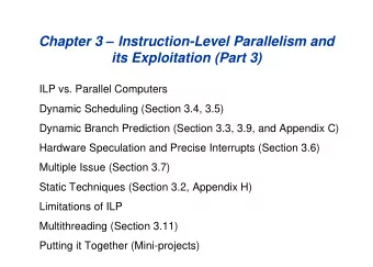
Chapter 3: Instruction Level Parallelism (ILP) and its exploitation - PDF document

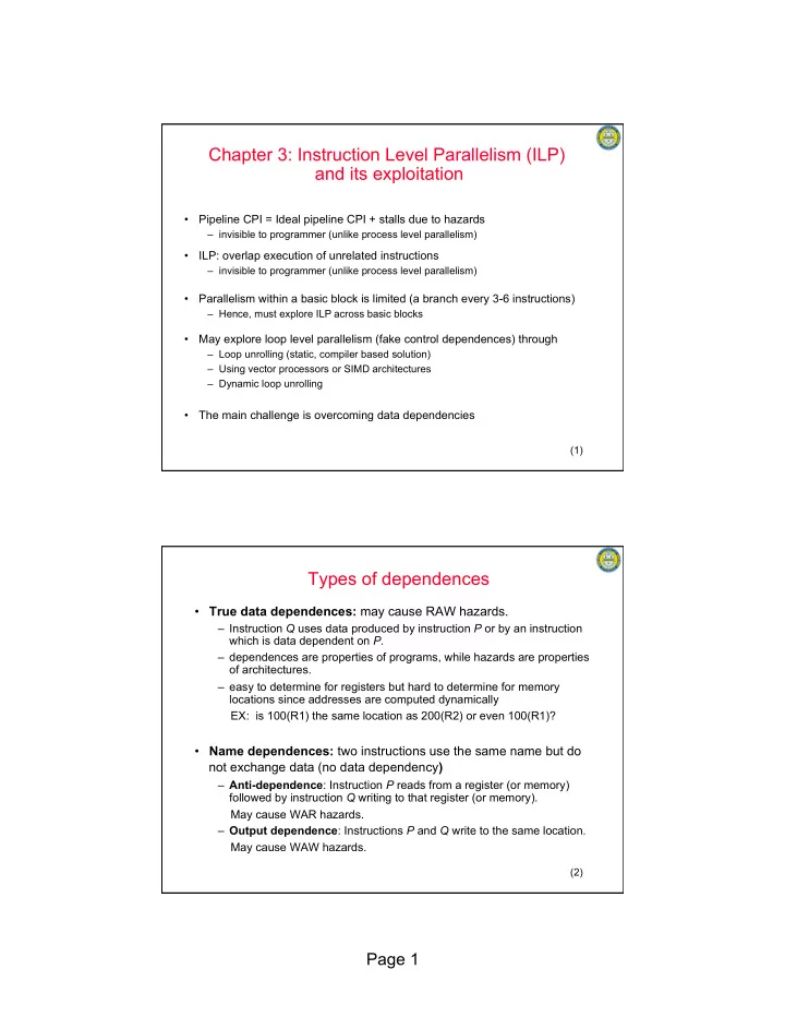
Chapter 3: Instruction Level Parallelism (ILP) and its exploitation • Pipeline CPI = Ideal pipeline CPI + stalls due to hazards – invisible to programmer (unlike process level parallelism) • ILP: overlap execution of unrelated instructions – invisible to programmer (unlike process level parallelism) • Parallelism within a basic block is limited (a branch every 3-6 instructions) – Hence, must explore ILP across basic blocks • May explore loop level parallelism (fake control dependences) through – Loop unrolling (static, compiler based solution) – Using vector processors or SIMD architectures – Dynamic loop unrolling • The main challenge is overcoming data dependencies (1) Types of dependences • True data dependences: may cause RAW hazards. – Instruction Q uses data produced by instruction P or by an instruction which is data dependent on P. – dependences are properties of programs, while hazards are properties of architectures. – easy to determine for registers but hard to determine for memory locations since addresses are computed dynamically EX: is 100(R1) the same location as 200(R2) or even 100(R1)? • Name dependences: two instructions use the same name but do not exchange data (no data dependency ) – Anti-dependence : Instruction P reads from a register (or memory) followed by instruction Q writing to that register (or memory) . May cause WAR hazards. – Output dependence : Instructions P and Q write to the same location. May cause WAW hazards. (2) Page 1

Loop: L.D F0, 0(R1) ADD.D F4, F0, F2 S.D 0(R1), F4 L.D F0, -8(R1) ADD.D F4, F0, F2 Data dependence S.D -8(R1), F4 Anti-dependence SUBI R1, R1, 16 Output dependence BNEZ R1, Loop How can you remove name dependences? Rename the dependent uses of F0 and F4 (3) Register renaming Loop: L.D F0, 0(R1) ADD.D F4, F0, F2 S.D 0(R1), F4 L.D F8, -8(R1) ADD.D F9, F8, F2 Data dependence S.D -8(R1), F9 Anti-dependence SUBI R1, R1, 16 Output dependence BNEZ R1, Loop How can you remove name dependences? Rename the dependent uses of F0 and F4 (4) Page 2

Control dependences • Determine the order of instructions with respect to branches. if P1 then S1 ; S1 is control dependent on P1 and if P2 then S2 ; S2 is control dependent on P2 (and P1 ??). • An instruction that is control dependent on P cannot be moved to a place where it is no longer control dependent on P , and visa-versa Example 1: Example 2: DADDU R1,R2,R3 DADDU R1,R2,R3 BEQZ R4,L BEQZ R12,skip DSUBU R1,R1,R6 DSUBU R4,R5,R6 L: … DADDU R5,R4,R9 OR R7,R1,R8 skip: OR R7,R8,R9 Possible to move DSUBU OR instruction depends before the branch (if R4 is not on the execution flow used after skip) (5) Loop carried dependences There is a loop carried dependence since For i=1,100 the statement in an iteration depends on a[i+1] = a[i] + c[i] ; an earlier iteration. For i=1,100 There is no loop carried dependence a[i] = a[i] + s ; • The iterations of a loop can be executed in parallel if there are no loop carried dependences . (6) Page 3

The effect of data dependencies (hazards) • Consider the following loop, which assumes that an array starts at location 8, with a number of elements (x 8) stored in register R1. Loop: L.D F0, 0(R1) ; Load an element ADD.D F4, F0, F2 ; add a scalar, in F2, to the element S.D F4, 0(R1) ; store result DADDUI R1, R1, #-8 ; update loop index, R1 BNE R1, R2, Loop ; branch if visited all elements • Assume a MIPS pipeline with the following latencies – Latency = 3 cycles if an FP ALU op follows an FP ALU op . – Latency = 2 cycles if an FP store follows an FP ALU op . – Latency = 1 cycle if an FP ALU op follows an FP load . BNE cond. – Latency = 1 cycle if a BNE follows an Integer ALU op. Evaluated in ID Int . IF ID Mem WB (7) FP FP FP FP Pipeline stalls due to data hazards Loop: L.D F0, 0(R1) ; Load an element stall ADD.D F4, F0, F2 ; add a scalar to the array element stall stall S.D F4, 0(R1) ; store result DADDUI R1, R1, #-8 ; update loop index, R1 stall BNE R1, R2, Loop ; branch if visited all elements 9 clock cycles per iteration (8) Page 4

Basic compiler techniques for exposing ILP (§3.2) Reorder the statements : Loop: L.D F0, 0(R1) DADDUI R1, R1, #-8 ADD.D F4, F0, F2 stall stall S.D F4, 8(R1) BNE R1, R2, Loop 7 clock cycles per iteration (9) Loop Unrolling (assume no pipelining) Loop: L.D F0, 0(R1) Loop: L.D F0, 0(R1) ADD.D F4, F0, F2 L.D F6, -8(R1) S.D F4, 0(R1) ADD.D F4, F0, F2 DADDUI R1, R1, #-8 ADD.D F8, F6, F2 L.D F0, 0(R1) DADDUI R1, R1, #-16 ADD.D F4, F0, F2 S.D F4, 16(R1) S.D F4, 0(R1) S.D F8, 8(R1) DADDUI R1, R1, #-8 BNE R1, R2, Loop BNE R1, R2, Loop Save 0.5 instruction per iteration Save 1 instruction per iteration • Need to worry about boundary cases (strip mining??) • Can reorder the statements if we use additional registers. • What limits the number of times we unroll a loop? • Note that loop iterations were independent for i = 1, 100 x(i) = x(i) + c (10) Page 5

Executing the unrolled loop on a pipeline Loop: L.D F0, 0(R1) L.D F6, -8(R1) ADD.D F4, F0, F2 ADD.D F8, F6, F2 DADDUI R1, R1, #-16 Problem if one cycle is required S.D F4, 16(R1) between integer op. and Store?. S.D F8, 8(R1) BNE R1, R2, Loop • Can solve the problem by • Stalling for one cycle • Replacing 16(R1) in the first SD statement by 0(R1). 4 clock cycles per iteration • What do you do if the latency = 3 cycles when S.D follows ADD.D? (11) Static branch prediction (§3.3) • Static branch prediction (built into the architecture) Ø The default is that branches are not taken Ø The default is that branches are taken • It is reasonable to assume that Ø forward branches are often not taken Ø backward branches are often taken • May come up with more accurate predictors based on branch directions. • Profiling is the standard technique for predicting the probability of branching. (12) Page 6

Dynamic Branch Prediction • Different than static branch predictions (predict taken or predict not taken). • Performance depends on the accuracy of prediction and the cost of miss-prediction. • Branch prediction buffer (Branch history table - BHT) : – 1-bit table (cache) indexed by the lower order bits of the address of the branch instructions (can be accessed in decode stage) – Says whether or not the branch was taken last time – needs to apply hashing techniques -- may have collision. – Will cause two miss-predictions in a loop (at start and end of loop). L1: …… . L2: …… . …… . BEQZ R2, L2 …… . BEQZ R1, L1 (13) Two bits branch predictors • change your prediction only if you miss-predict twice • helps if a branch changes directions occasionally (ex. Nested loops) 1 1 1 0 Branch taken Predict taken Predict taken Branch not taken Predict not taken Predict not taken 0 0 0 1 • In general, n -bit predictors are called Local Predictors . – Use a saturated counter (++ on correct prediction, -- on wrong prediction) – n-bit prediction is not much better than 2-bit prediction (n > 2). – A BHT with 4K entries is as good as an infinite size BHT – Dynamic branch prediction does not help in the 5-stage pipeline (why?) – Miss-predict when gets the wrong branch in BHT or a wrong prediction. (14) Page 7

Correlating Branch predictors (global predictors) • Hypothesis: recent branches are correlated (behavior of recently executed branches affects prediction of current branch). SUBUI R3,R1,2 • Example 1: if (a == 2) BNEZ R3, L1 … B1 a = 0 ; ADD R1, R0, R0 if (b == 2) L1: SUBUI R3, R2, 2 b = 0; BNEZ R3, L2 B2 ADD R2, R0, R0 if (a != b) ... L2: SUBU R3, R1, R2 BNEZ R3, L3 B3 If B1 and B2 are taken, then B3 will probably not be taken, If B1 and B2 are not taken, the B3 is taken • Example 2: If (d == 0) d = 1 ; if (d == 1) ..... (15) Correlating Branch predictors • Keep history of the m most recently executed branches in an m -bit shift register. • Record the prediction for each branch instruction, and each of the 2 m combinations. • In general, ( m,n ) predictor means record last m branches to select between 2 m history tables each with n -bit predictor. • Simple access scheme (double indexing). • A ( 0,n ) predictor is a local n -bit predictor. • Size of table is N n 2 m , where N is the number of table entries. • There is a tradeoff between N (determines A (2,2) predictor collision), n (accuracy of local predicion) and m (determines history). (16) Page 8

Tournament predictor (hybrid local-global predictors) • Combines a global predictor and a local predictor with a strategy for selecting the appropriate predictor (multilevel predictors). 1/0, 0/0, 1/1 0/1, 0/0, 1/1 Use predictor 1 Use predictor 2 0/1 1/0 1/0 0/1 0/1 Use predictor 1 Use predictor 2 0/0, 1/1 0/0, 1/1 1/0 p 1 /p 2 == predictor 1 is correct/predictor 2 is correct • The Alpha 21264 selects between – a (12,2) global predictor with 4K entries – a local predictor which selects a prediction based on the outcome of the last 10 executions of any given branch. (17) Performance of Branch predictors (18) Page 9