[PPT] - Chapter 11. Stochastic Methods Rooted in Statistical Mechanics PowerPoint Presentation

SLIDE 1

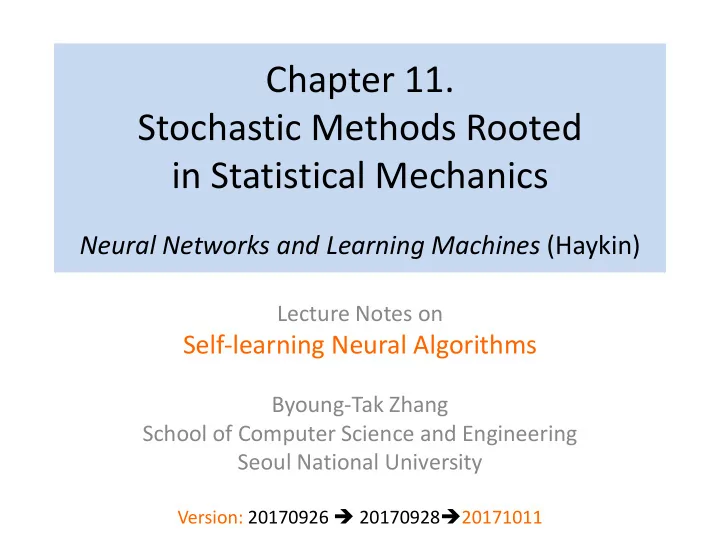
Chapter 11. Stochastic Methods Rooted in Statistical Mechanics

Neural Networks and Learning Machines (Haykin)

Lecture Notes on

Self-learning Neural Algorithms

Byoung-Tak Zhang School of Computer Science and Engineering Seoul National University

Version: 20170926 è 20170928è20171011

SLIDE 2

11.1 Introduction …………………………………………………………………………….... 3 11.2 Statistical Mechanics ……………………………………………………………..…. 4 11.3 Markov Chains ………………………..………………………………………..…….... 6 11.4 Metropolis Algorithm ……….………..………………….……………………..... 16 11.5 Simulated Annealing ………………………………………………….…….…...…. 19 11.6 Gibbs Sampling ….…………….…….………………..……..……………………….. 22 11.7 Boltzmann Machine …..……………………………………….……..…………….. 24 11.8 Logistic Belief Nets ……………….…………………..……………….…......……. 29 11.9 Deep Belief Nets ………………………….…………………………..….........…. 30 11.10 Deterministic Annealing (DA) …………….………………………..…….…... 34 11.11 Analogy of DA with EM …..……….….…………………………………….……. 39 Summary and Discussion …………….…………….………………………….………... 41

SLIDE 3

11.1 Introduction

Statistical mechanics as a source of ideas for unsupervised (self-
rganized) learning systems
Statistical mechanics

ü The formal study of macroscopic equilibrium properties of large systems of elements that are subject to the microscopic laws of mechanics. ü The number of degrees of freedom is enormous, making the use of probabilistic methods mandatory. ü The concept of entropy plays a vital role in statistical mechanics, as with the Shannon’s information theory. ü The more ordered the system, or the more concentrated the underlying probability distribution, the smaller the entropy will be.

Statistical mechanics for the study of neural networks

ü Cragg and Temperley (1954) and Cowan (1968) ü Boltzmann machine (Hinton and Sejnowsky, 1983, 1986; Ackley et al., 1985)

SLIDE 4

11.2 Statistical Mechanics (1/2)

! pi :!probability!of!occurrence!of!state!i!of!a!stochastic!system !!!!!pi ≥0!(for!all!i)!!and! pi

i

∑

=1 Ei :!energy!of!the!system!when!it!is!in!state!i In!thermal!equilibrium,!the!probability!of!state!i!is (Canonical!distribution!/!Gibbs!distribution) !!!!!pi = 1 Z exp − Ei kBT ⎛ ⎝ ⎜ ⎞ ⎠ ⎟ !!!!!Z = exp − Ei kBT ⎛ ⎝ ⎜ ⎞ ⎠ ⎟

i

∑

exp −E /kBT

( ):!Boltzmann!factor!

Z :!sum!over!states!(partition!function) We!set!kB =1!and!view!−logpi !as!"energy"

1. States of low energy have a higher

probability of occurrence than the states of high energy.

2. As the temperature T is reduced, the

probability is concentrated on a smaller subset of low-energy states.

SLIDE 5

11.2 Statistical Mechanics (2/2)

! Helmholtz!free!energy !!!!!!!F = −TlogZ < E > ! = piEi

i

∑

!!!!!!(avergage!energy) !!!!!! < E > −!F = −T pi logpi

i

∑

H = − pi logpi

i

∑

!!!!!(entropy) Thus,!we!have !!!!!! < E > −!F =TH !!!!!!!F = ! < E > −!TH Consider!two!systems!A!and!A'!in!thermal!contact. ΔH!and!ΔH':!entropy!changes!of!A!and!A'! The!total!entropy!tends!to!increase!with !!!!!!!ΔH + ΔH'≥0

! The!free!energy!of!the!system,!F,!tends!to!decrease!and become!a!minimum!in!an!equilibrium!situation.! The!resulting!probability!distribution!is!defined!by! Gibbs!distribution!(The!Principle!of!Minimum!Free!Energy).!

Nature likes to find a physical system with minimum free energy.

SLIDE 6

Markov property P(X n+1 = xn+1 | X n = xn,…, X1 = x1) = P(X n+1 = xn+1 | X n = xn) Transition probability from state i at time n to j at time n +1 pij = P(X n+1 = j | X n = i) (pij ≥ 0 ∀i, j and pij = 1 ∀i

j

∑

) If the transition probabilities are fixed, the Markov chain is homogeneous. In case of a system with a finite number of possible states K, the transition probabilities constitute a K-by-K matrix (stochastic matrix): P = p11 … p1K ! " ! pK1 # pKK ⎛ ⎝ ⎜ ⎜ ⎜ ⎞ ⎠ ⎟ ⎟ ⎟

11.3 Markov Chains (1/9)

SLIDE 7

11.3 Markov Chains (2/9)

Generalization to m-step transition probability pij

(m) = P(X n+m = x j | X n = xi),

m = 1,2,… pij

(m+1) =

pik

(m) pkj,

m = 1,2,…, pik

(1) = pik k

∑

We can further generalize to (Chapman-Kolmogorov identity) pij

(m+n) =

pik

(m) pkj (n) k

∑

, m,n = 1,2,…

lim

k→∞vi(k) = π i

i = 1,2,…,K

SLIDE 8

11.3 Markov Chains (3/9)

Properties of markov chains Recurrent pi = P(every returning to state i) Transient pi <1 Periodic If i ∈Sk and pi > 0, then j ∈Sk+1, for k = 1,...,d -1 j ∈Sk, for k = 1,...,d ⎧ ⎨ ⎪ ⎩ ⎪ Aperiodic Accessable: Accessable from i if there is a finite sequence of transition from i to j Communicate: If the states i and j are accessible to each other If two states communicate each other, they belong to the same class. If all the states consists of a single class, the Markov chain is indecomposible or irreducible.

SLIDE 9

11.3 Markov Chains (4/9)

Figure 11.1: A periodic recurrent Markov chain with d = 3.

SLIDE 10

11.3 Markov Chains (5/9)

Ergodic Markov chains Ergodicity: time average = ensemble average i.e. long-term proportion of time spent by the chain in state i corresponds to the steady-state probability π i vi(k): Proportion of time spent in state i after k returns vi(k) = k Ti(ℓ)

ℓ=1 k

∑

lim

k→∞vi(k) = π i

i = 1,2,…,K

SLIDE 11

11.3 Markov Chains (6/9)

Convergence to Stationary Distributions Consider an ergodic Markov chain with a stochastic matrix P π (n−1) : state transition vector of the chain at time n-1 State transition vector at time n is π (n) = π (n−1)P By iteration we obtain π (n) = π (n−1)P = π (n−2)P2 = π (n−3)P3 =! π (n) = π (0)Pn π (0) : initial value lim

n→∞Pn =

π1 … π K " # " π1 ! π K ⎛ ⎝ ⎜ ⎜ ⎜ ⎞ ⎠ ⎟ ⎟ ⎟ = π " π ⎛ ⎝ ⎜ ⎜ ⎜ ⎞ ⎠ ⎟ ⎟ ⎟

Ergodic theorem

1. lim

n→∞ pij (n) = π j

∀i

2. π j > 0

∀j 3. π j = 1

j=1 K

∑

4. π j =

π i pij

i=1 K

∑

for j = 1,2,…,K

SLIDE 12

11.3 Markov Chains (6/9)

Figure 11.2: State-transition diagram of Markov chain for Example 1: The states x1 and x2 and may be identified as up-to-date behind, respectively.

12

! P = 1 4 3 4 1 2 1 2 ⎡ ⎣ ⎢ ⎢ ⎢ ⎢ ⎤ ⎦ ⎥ ⎥ ⎥ ⎥ ! π (0) = 1 6 5 6 ⎡ ⎣ ⎢ ⎢ ⎤ ⎦ ⎥ ⎥ π (1) = π (1)P !!!!!!! = ! 1 6 5 6 ⎡ ⎣ ⎢ ⎢ ⎤ ⎦ ⎥ ⎥ 1 4 3 4 1 2 1 2 ⎡ ⎣ ⎢ ⎢ ⎢ ⎢ ⎤ ⎦ ⎥ ⎥ ⎥ ⎥ !!!!!! = ! 11 24 13 24 ⎡ ⎣ ⎢ ⎢ ⎤ ⎦ ⎥ ⎥

! P(2) = 0.4375 0.5625 0.3750 0.6250 ⎡ ⎣ ⎢ ⎤ ⎦ ⎥ P(3) = 0.4001 0.5999 0.3999 0.6001 ⎡ ⎣ ⎢ ⎤ ⎦ ⎥ P(4) = 0.4000 0.6000 0.4000 0.6000 ⎡ ⎣ ⎢ ⎤ ⎦ ⎥

SLIDE 13

11.3 Markov Chains (7/9)

Figure 11.3: State-transition diagram of Markov chain for Example 2.

! P = 1 1 3 1 6 1 2 3 4 1 4 ⎡ ⎣ ⎢ ⎢ ⎢ ⎢ ⎢ ⎢ ⎢ ⎤ ⎦ ⎥ ⎥ ⎥ ⎥ ⎥ ⎥ ⎥

! π1 = 1 3π2 + 3 4π3 π2 = 1 6π2 + 1 4π3 π3 = π1 + 1 2π2

π j = π i pij

i=1 K

∑

! π1 = 0.3953 π2 = 0.1395 π3 = 0.4652

SLIDE 14

11.3 Markov Chains (8/9)

Figure 11.4: Classification of the states of a Markov chain and their associated long-term behavior.

14

SLIDE 15

11.3 Markov Chains (9/9)

Principle of detailed balance At thermal equilibrium, the rate of occurrence of any transition equals the corresponding rate of occurrence of the inverse transition, πi pij = π j p ji Application :stationary distribution πi pij

i=1 K

∑

= πi π j pij ⎛ ⎝ ⎜ ⎞ ⎠ ⎟

i=1 K

∑

π j = π j π j p ji ⎛ ⎝ ⎜ ⎞ ⎠ ⎟

i=1 K

∑

π j = p ji

( )

i=1 K

∑

π j (πi pij = π j p ji,detailed balance) = π j (since p ji

i=1 K

∑

=1)

SLIDE 16

11.4 Metropolis Algorithm (1/3)

Metropolis Algorithm A stochastic algorithm for simulating the evolution of a physical system to thermal equilibrium. A modified Monte Carlo method. Markov Chain Monte Carlo (MCMC) method Algorithm Metropolis

1. X n = xi. Randomly generate a new state x j.
2. ΔE = E(x j) − E(xi)
3. If ΔE < 0, then X n+1 = x j

else if ΔE ≥ 0, then { Select a random number ξ ∼ U[0,1]. If ξ < exp(−ΔE / T), then X n+1 = x j, (accept) else X n+1 = xi. (reject) }

SLIDE 17

11.4 Metropolis Algorithm (2/3)

Choice of Transition Probabilities Proposed set of transition probabilities

1. τ ij > 0 (for all i, j) : Nonnegativity

2. τ ij

j

∑

=1 (for all i) : Normalization

3. τ ij = τ ji (for all i, j) : Symmetry

Desired set of transition probabilities pij = τ ij π j πi ⎛ ⎝ ⎜ ⎞ ⎠ ⎟ for π j πi <1 τ ij for π j πi ≥1 ⎧ ⎨ ⎪ ⎪ ⎪ ⎩ ⎪ ⎪ ⎪ pii = τ ii + τ ij 1− π j πi ⎛ ⎝ ⎜ ⎞ ⎠ ⎟ =1− αijτ ij

j≠i

∑

j≠i

∑

Moving probability α ij = min 1, π j π i ⎛ ⎝ ⎜ ⎞ ⎠ ⎟

SLIDE 18

11.4 Metropolis Algorithm (3/3)

How to choose the ratio π j / π i ? We choose the probability distribution to which we want the Markov chain to coverge to be a Gibbs distribution π j = 1 Z exp − E j T ⎛ ⎝ ⎜ ⎞ ⎠ ⎟ π j π i = exp − ΔE T ⎛ ⎝ ⎜ ⎞ ⎠ ⎟ ΔE = E j − Ei Proof of detailed balance : Case 1: ΔE < 0. π i pij = π iτ ij = π iτ ji π j p ji = π j π i π j τ ji ⎛ ⎝ ⎜ ⎞ ⎠ ⎟ = π iτ ji Case 2: ΔE > 0. π i pij = π i π j π i τ ij ⎛ ⎝ ⎜ ⎞ ⎠ ⎟ = π jτ ji π j p ji = π iτ ij

SLIDE 19

11.5 Simulated Annealing (1/3)

Simulated Annealing

A stochastic relaxation technique for solving optimization problems.
Improves the computational efficiency of the Metropolis algorithm.
Makes random moves on the energy surface
Operate a stochastic system at a high temperature (where convergence to

equilibrium is fast) and then iteratively lower the temperature (at T=0, the Markov chain collapses on the global minima). Two ingredients: 1. A schedule that determines the rate at which the temperature is lowered. 2. An algorithm, such as the Metropolis algorithm, that iteratively finds the equilibrium distribution at each new temperature in the schedule by using the final state of the system at the previous temperature as the starting point for the new temperature.

! F = ! < E > −TH,!!!!!!lim

T→0 !F! = ! < E >

SLIDE 20

11.5 Simulated Annealing (2/3)

1. Initial Value of the Temperature. The initial value T0 of the temperature is chosen high enough to ensure that virtually all proposed transitions are accepted by the simulated-annealing algorithm 2. Decrement of the Temperature. Ordinarily, the cooling is performed exponentially, and the changes made in the value of the temperature are

small. In particular, the decrement function is defined by

where α is a constant smaller than, but close to, unity. Typical values of α lie between 0.8 and 0.99. At each temperature, enough transitions are attempted so that there are 10 accepted transitions per experiment, on average. 3. Final Value of the Temperature. The system is fixed and annealing stops if the desired number of acceptances is not achieved at three successive temperatures Tk = αTk−1, k = 1,2,…,K

SLIDE 21

11.5 Simulated Annealing (3/3)

Simulated Annealing for Combinatorial Optimization

SLIDE 22

11.6 Gibbs Sampling (1/2)

22

Gibbs sampling An iterative adaptive scheme that generates a single value for the conditional distribution for each component of the random vector X, rather than all values of the variables at the same time. X = X1, X2,..., X K : a random vector of K components Assume we know P(X k | X−k ),where X−k = X1, X2,..., X k−1X k+1,..., X K Gibbs sampling algorithm (Gibbs sampler)

1. Initialize x1(0),x2(0),...,xK(0).
2. i ←1

3. If (termination condition not met), then i ← i +1 and go to step 2.

SLIDE 23

11.6 Gibbs Sampling (2/2)

1. Convergence theorem. The random variable X k(n) converges in distribution to the true

probability distributions of X k for k = 1, 2, ..., K as n approaches infinity; that is, lim

n→∞ P(X k (n) ≤ x | xk(0)) = P Xk (x)

for k = 1,2,…,K where P

Xk (x) is marginal cumulative distribution function of X k.

2. Rate-of-convergence theorem. The joint cumulative distribution of the random

variables X1(n), X2(n), ..., X K(n) converges to the true joint cumulative distribution

f X1, X2, ..., X K at a geometric rate in n.
3. Ergodic theorem. For any measurable function g of the random variables

X1, X2, ..., X K whose expectation exists, we have lim

n→∞

1 n g(X1(i), X2(i),…, X K(i)) → E[g(X1, X2,…X K )]

i=1 n

∑

with probability 1 (i.e., almost surely).

SLIDE 24

11.7 Boltzmann Machine (1/5)

Figure 11.5: Architectural graph of Boltzmann machine; K is the number of visible neurons, and L is the number of hidden neurons. The distinguishing features of the machine are:

1. The connections between the visible and hidden neurons are symmetric.
2. The symmetric connections are extended to the visible and hidden neurons.

24

Boltzmann machine (BM) x : state vector of BM wji : synaptic connection from i to j Structure (weights) wji = wij ∀i, j wii = 0 ∀i Energy E(x) = − 1 2 wjixix j

j≠i

∑

i

∑

Probability P(X = x) = 1 Z exp − E(x) T ⎛ ⎝ ⎜ ⎞ ⎠ ⎟

A stochastic machine consisting of stochastic neurons with symmetric synaptic connections.

SLIDE 25

11.7 Boltzmann Machine (2/5)

Consider three events: A: X j = x j B : Xi = xi

{ }i=1

K with i ≠ j

C : Xi = xi

{ }i=1

K

The joint event B excludes A, and the joint event C includes both A and B. P(C) = P(A,B) = 1 Z exp 1 2T wjixix j

j, j≠i

∑

i

∑

⎛ ⎝ ⎜ ⎞ ⎠ ⎟ P(B) = P(A,B)

A

∑

= 1 Z exp 1 2T wjixix j

j, j≠i

∑

i

∑

⎛ ⎝ ⎜ ⎞ ⎠ ⎟

x j

∑

The component involving x j x j 2T wjixi

i≠ j

∑

P(A| B) = P(A,B) P(B) = 1 1+ exp − x j T wjixi

i i≠ j

∑

⎛ ⎝ ⎜ ⎜ ⎞ ⎠ ⎟ ⎟ P X j = x | Xi = xi

{ }i=1,i≠ j

K

( ) = ϕ

x T wjixi

i,i≠ j K

∑

⎛ ⎝ ⎜ ⎞ ⎠ ⎟ ϕ(v) = 1 1+ exp(−v)

SLIDE 26

11.7 Boltzmann Machine (3/5)

Figure 11.6: Sigmoid-shaped function P(v).

L(w) = log P(Xα = xα )

xα ∈ ℑ

∏

= log P(Xα = xα )

xα ∈ ℑ

∑

1. Positive phase. In this phase, the network
perates in its clamped condition (i.e.,under

the direct influence of the training sample ).

2. Negative phase. In this second phase, the

network is allowed to run freely, and therefore with no environmental input. 𝕶

SLIDE 27

11.7 Boltzmann Machine (4/5)

xα : the state of the visible neurons (subset of x) xβ : the state of the hidden neurons (subset of x) Probability of the visible state P(Xα = xα ) = 1 Z exp − E(x) T ⎛ ⎝ ⎜ ⎞ ⎠ ⎟

xβ

∑

Z = exp − E(x) T ⎛ ⎝ ⎜ ⎞ ⎠ ⎟

x

∑

Log-likelihood function given the training data ℑ L(w) = log P(x | w) = log exp − E(x) T ⎛ ⎝ ⎜ ⎞ ⎠ ⎟

xβ

∑

− log exp − E(x) T ⎛ ⎝ ⎜ ⎞ ⎠ ⎟

x

∑

⎛ ⎝ ⎜ ⎞ ⎠ ⎟

xα ∈ ℑ

∑

Derivative of the log-likelihood function ∂L(w) ∂wji = 1 T P(Xβ = xβ | Xα = xα )

xβ

∑

x jxi − P(X = x)x jxi

x

∑

( )

xα ∈ ℑ

∑

SLIDE 28

11.7 Boltzmann Machine (5/5)

Mean firing rate in the positive phase (clamped) ρ ji

+ = x jxi +

= P(X = xβ | X = xα )x jxi

xβ

∑

xα ∈ℑ

∑

Mean firing rate in the negative phase (free-running) ρ ji

− = x jxi −

= P(X = x)x jxi

x

∑

xα ∈ℑ

∑

Thus, we may write ∂L(w) ∂w ji = 1 T (ρ ji

+ − ρ ji − )

Gradient ascent to maximize the L(w) Δw ji = η ∂L(w) ∂w ji = η'(ρ ji

+ − ρ ji − )

η' = ε T Boltzmann machine learning rule

SLIDE 29

11.8 Logistic Belief Nets

Figure 11.7: Directed (logistic) belief network.

Parents of node j pa(X j) ⊆ X1, X2,…, X j−1

{ }

Conditional probability P(X j = x j | X1 = x1,…, X j−1 = x j−1) = P(X j = x j | pa(X j))

A stochastic machine consisting of multiple layers of stochastic neurons with directed synaptic connections.

Calculation of conditional probabilities

1. wji = 0 for all Xi ∉ pa(X j)
2. wji = 0 for i ≥ j (∵acyclic)

Weight update rule Δwji = η ∂ ∂wji L(w)

SLIDE 30

11.9 Deep Belief Nets (1/4)

Figure 11.8: Neural structure of restricted Boltzmann machine (RBM). Contrasting this with that of Fig. 11.6, we see that unlike the Boltzmann machine, there are no connections among the visible neurons and the hidden neurons in the RBM.

Maximum-Likelihood Learning in a Restricted Boltzmann Machine (RBM)

Sequential pre - training

1. Update the hidden states h in parallel,

given the visible states x.

2. Doing the same, but in reverse:

update the visible states x in parallel, given the hidden states h. Maximum - likelihood learning ∂L(w) ∂wji = ρ ji

(0) − ρ ji (∞)

SLIDE 31

11.9 Deep Belief Nets (2/4)

Figure 11.9: Top-down learning, using logistic belief network of infinite depth.

31

Figure 11.10: A hybrid generative model in which the two top layers form a restricted Boltzmann machine and the lower two layers form a directed

model. The weights shown with blue shaded

arrows are not part of the generative model; they are used to infer the feature values given to the data, but they are not used for generating data.

SLIDE 32

11.9 Deep Belief Nets (3/4)

Figure 11.11: Illustrating the progression of alternating Gibbs

sampling in an RBM. After sufficiently many steps, the visible and hidden

vectors are sampled from the stationary distribution defined by the current parameters of the model.

SLIDE 33

11.9 Deep Belief Nets (4/4)

Figure 11.12: The task of modeling the sensory (visible) data is divided into two subtasks.

SLIDE 34

11.10 Deterministic Annealing (1/5)

Deterministic Annealing Incorporates randomness into the energy function, which is then deterministically optimized at a sequence of decreasing temperature (cf. simulated annealing: random moves on the energy surface) Clustering via Deterministic Annealing x :source (input) vector y :reconstruction (output) vector Distortion measure: d(x,y) = x − y

2

Expected distortion: D = P(X = x,Y = y)d(x,y)

y

∑

x

∑

= P(X = x) P(Y = y | X = x)d(x,y)

y

∑

x

∑

Probability of joint event P(X = x,Y = y) = P(Y = y | X = x)

association probability

! " ## $ ## P(X = x)

SLIDE 35

11.10 Deterministic Annealing (2/5)

Table 11.2

Entropy as randomness measure H(X,Y) = − P(X = x,Y = y)log P(X = x,Y = y)

y

∑

x

∑

Constrained optimization of D as minimization of the Lagrangean F = D −TH H(X,Y) = H(X)

source entropy

! + H(Y | X)

conditional entropy

! " # $ # H(Y | X) = − P(X = x) P(Y = y | X = x)log P(Y = y | X = x)

y

∑

x

∑

P(Y = y | X = x) = 1 Zx exp − d(x,y) T ⎛ ⎝ ⎜ ⎞ ⎠ ⎟ , Zx = exp − d(x,y) T ⎛ ⎝ ⎜ ⎞ ⎠ ⎟

y

∑

SLIDE 36

11.10 Deterministic Annealing (3/5)

F * = min

P(Y=y|X=x) F

= −T P(X = x)logZx

x

∑

Setting ∂ ∂y F * = P(X = x,Y = y) ∂ ∂y d(x,y)

x

∑

= 0 ∀y ∈ϒ The minimizing condition is 1 N P(Y = y | X = x)

x

∑

∂ ∂y d(x,y) = 0 ∀y ∈ϒ The deterministic annealing algorithm consists of minimizing the Lagrangian F * with respect to the code vectors at a high value of temperature T and then tracking the minimum while the temperature T is lowered.

SLIDE 37

11.10 Deterministic Annealing (4/5)

Figure 11.13: Clustering at various phases. The lines are equiprobability contours, p = ½ in (b), and p = ⅓ elsewhere: (a) 1 cluster (B = 0), (b) 2 clusters (B = 0.0049), (c) 3 clusters (B = 0.0056), (d) 4 clusters (B = 0.0100), (e) 5 clusters (B = 0.0156), (f) 6 clusters (B = 0.0347), and (g) 19 clusters (B = 0.0605). 37 (c) 2017 Biointelligence Lab, SNU

! B = 1 T

SLIDE 38

11.10 Deterministic Annealing (5/5)

Figure 11.14: Phase diagram for the Case Study in deterministic annealing. The number of effective clusters is shown for each phase.

! B = 1 T

SLIDE 39

11.11 Analogy of DA with EM (1/2)

Suppose we view the association probability P(Y = y | X = x) as the expected value of a random binary variable Vxy defined as Vxy 1 if thesourcevectorxisassigned tocodevector y

therwise

⎧ ⎨ ⎪ ⎩ ⎪ Then, the two steps of DA = two steps of EM

1. Step 1 of DA (= E-step of EM)

Compute the association probabilities P(Y = y | X = x)

2. Step 2 of DA (= M-step of EM)

Optimize the distortion measure d(x,y)

SLIDE 40

11.11 Analogy of DA with EM (2/2)

r : complete data including missing data z d = d(r): incomplete data Conditional pdf of r given param vector θ pD(d | θ) = pc(r | θ)dr

ℜ(d )

∫

ℜ(d): subspace of ℜ determined by d = d(r) Incomplete log-likelihood function L(θ) = log pD(d | θ) Complete-data log-likelihood function Lc(θ) = log pc(r | θ)

Expectation - Maximization Algorithm ˆ θ(n): value of θ at iteration n of EM

1. E-step

Q(θ, ˆ θ(n)) = Eˆ

θ(n) LC(θ)

⎡ ⎣ ⎤ ⎦

2. M-step

ˆ θ(n +1) = argmax

θ

Q(θ, ˆ θ(n)) After an interation of the EM algorithm, the incomplete-data log-likelihood function is not decreased: L(ˆ θ(n +1) ≥ L(ˆ θ(n)) for n = 0,1,2,…,K

SLIDE 41

Chapter 11. Stochastic Methods Rooted in Statistical Mechanics

Neural Networks and Learning Machines (Haykin)

Lecture Notes on

Self-learning Neural Algorithms

Byoung-Tak Zhang School of Computer Science and Engineering Seoul National University

Contents

11.1 Introduction

11.2 Statistical Mechanics (1/2)

∑

∑

( ):!Boltzmann!factor!

11.2 Statistical Mechanics (2/2)

∑

∑

∑

∑

11.3 Markov Chains (1/9)

11.3 Markov Chains (2/9)

Generalization to m-step transition probability pij

m = 1,2,… pij

pik

m = 1,2,…, pik

∑

We can further generalize to (Chapman-Kolmogorov identity) pij

pik

∑

, m,n = 1,2,…

11.3 Markov Chains (3/9)

11.3 Markov Chains (4/9)

11.3 Markov Chains (5/9)

∑

11.3 Markov Chains (6/9)

∑

∑

11.3 Markov Chains (6/9)

11.3 Markov Chains (7/9)

∑

11.3 Markov Chains (8/9)

11.3 Markov Chains (9/9)

∑

∑

∑

( )

∑

∑

11.4 Metropolis Algorithm (1/3)

11.4 Metropolis Algorithm (2/3)

∑

∑

∑

11.4 Metropolis Algorithm (3/3)

11.5 Simulated Annealing (1/3)

Simulated Annealing

! F = ! < E > −TH,!!!!!!lim

11.5 Simulated Annealing (2/3)

11.5 Simulated Annealing (3/3)

Simulated Annealing for Combinatorial Optimization

11.6 Gibbs Sampling (1/2)

11.6 Gibbs Sampling (2/2)

∑

11.7 Boltzmann Machine (1/5)

∑

∑

11.7 Boltzmann Machine (2/5)

{ }i=1

{ }i=1

∑

∑

∑

∑

∑

∑

∑

∑

{ }i=1,i≠ j

( ) = ϕ

∑

11.7 Boltzmann Machine (3/5)

∏

∑