Chapter 10 Verification and Validation of Simulation Models Banks, - PowerPoint PPT Presentation
Chapter 10 Verification and Validation of Simulation Models Banks, Carson, Nelson & Nicol Discrete-Event System Simulation Purpose & Overview The goal of the validation process is: To produce a model that represents true
Chapter 10 Verification and Validation of Simulation Models Banks, Carson, Nelson & Nicol Discrete-Event System Simulation
Purpose & Overview The goal of the validation process is: To produce a model that represents true behavior closely enough for decision-making purposes To increase the model ’ s credibility to an acceptable level Validation is an integral part of model development Verification – building the model correctly (correctly implemented with good input and structure) Validation – building the correct model (an accurate representation of the real system) Most methods are informal subjective comparisons while a few are formal statistical procedures 2
Model-Building, Verification & Validation 3
Verification Purpose: ensure the conceptual model is reflected accurately in the computerized representation. Many common-sense suggestions, for example: Have someone else check the model. Make a flow diagram that includes each logically possible action a system can take when an event occurs. Closely examine the model output for reasonableness under a variety of input parameter settings. Print the input parameters at the end of the simulation, make sure they have not been changed inadvertently. 4
Examination of Model Output for Reasonableness [Verification] Example: A model of a complex network of queues consisting many service centers. Response time is the primary interest, however, it is important to collect and print out many statistics in addition to response time . Two statistics that give a quick indication of model reasonableness are current contents and total counts , for example: If the current content grows in a more or less linear fashion as the simulation run time increases, it is likely that a queue is unstable If the total count for some subsystem is zero, indicates no items entered that subsystem, a highly suspect occurrence If the total and current count are equal to one, can indicate that an entity has captured a resource but never freed that resource. Compute certain long-run measures of performance, e.g. compute the long-run server utilization and compare to simulation results 5
Other Important Tools [Verification] Documentation A means of clarifying the logic of a model and verifying its completeness Use of a trace A detailed printout of the state of the simulation model over time. 6
Calibration and Validation Validation: the overall process of comparing the model and its behavior to the real system. Calibration: the iterative process of comparing the model to the real system and making adjustments. 7
Calibration and Validation No model is ever a perfect representation of the system The modeler must weigh the possible, but not guaranteed, increase in model accuracy versus the cost of increased validation effort. Three-step approach: Build a model that has high face validity. Validate model assumptions. Compare the model input-output transformations with the real system ’ s data. 8
High Face Validity [Calibration & Validation] Ensure a high degree of realism: Potential users should be involved in model construction (from its conceptualization to its implementation). Sensitivity analysis can also be used to check a model ’ s face validity. Example: In most queueing systems, if the arrival rate of customers were to increase, it would be expected that server utilization, queue length and delays would tend to increase. 9
Validate Model Assumptions [Calibration & Validation] General classes of model assumptions: Structural assumptions: how the system operates. Data assumptions: reliability of data and its statistical analysis. Bank example: customer queueing and service facility in a bank. Structural assumptions, e.g., customer waiting in one line versus many lines, served FCFS versus priority. Data assumptions, e.g., interarrival time of customers, service times for commercial accounts. Verify data reliability with bank managers. Test correlation and goodness of fit for data (see Chapter 9 for more details). 10
Validate Input-Output Transformation [Calibration & Validation] Goal: Validate the model ’ s ability to predict future behavior The only objective test of the model. The structure of the model should be accurate enough to make good predictions for the range of input data sets of interest. One possible approach: use historical data that have been reserved for validation purposes. Criteria: use the main responses of interest. 11
Bank Example [Validate I-O Transformation] Example: One drive-in window serviced by one teller, only one or two transactions are allowed. Data collection: 90 customers during 11 am to 1 pm. Observed service times {S i , i = 1,2, … , 90} . Observed interarrival times {A i , i = 1,2, … , 90} . Data analysis let to the conclusion that: Interarrival times: exponentially distributed with rate l = 45 Service times: N(1.1, 0.2 2 ) 12
Bank Example [Validate I-O Transformation] 13
Bank Example [Validate I-O Transformation] 14
The Black Box [Bank Example: Validate I-O Transformation] A model was developed in close consultation with bank management and employees Model assumptions were validated Resulting model is now viewed as a “ black box ” : Model Output Variables, Y Input Variables Primary interest: Y 1 = teller ’ s utilization Possion arrivals l = 45/hr: X 11 , X 12 , … Y 2 = average delay Uncontrolled Y 3 = maximum line length Services times, Model variables, X “ black box ” N(D 2 , 0.22): X 21 , X 22 , … Secondary interest: f(X,D) = Y Y 4 = observed arrival rate D 1 = 1 (one teller) Controlled Y 5 = average service time D 2 = 1.1 min Decision Y 6 = sample std. dev. of (mean service time) variables, D service times D 3 = 1 (one line) Y 7 = average length of time 15
Comparison with Real System Data [Bank Example: Validate I-O Transformation] Real system data are necessary for validation. System responses should have been collected during the same time period (from 11 am to 1 pm on the same Friday.) Compare the average delay from the model Y 2 with the actual delay Z 2 : Average delay observed, Z 2 = 4.3 minutes, consider this to be the true mean value m 0 = 4.3. When the model is run with generated random variates X 1n and X 2n , Y 2 should be close to Z 2 . Six statistically independent replications of the model, each of 2- hour duration, are run. 16
Results of Six Replications of the First Bank Model [Bank Example: Validate I-O Transformation] Y4 Y5 Y2 =Average Delay Replication (Arrival/Hour) ( Minutes ) ( Minutes ) 1 51 1.07 2.79 2 40 1.12 1.12 3 45.5 1.06 2.24 4 50.5 1.10 3.45 5 53 1.09 3.13 6 49 1.07 2.38 Sample mean 2.51 Standard deviation 0.82 17
Hypothesis Testing [Bank Example: Validate I-O Transformation] Compare the average delay from the model Y 2 with the actual delay Z 2 (continued): Null hypothesis testing: evaluate whether the simulation and the real system are the same (w.r.t. output measures): H : E(Y ) 4 . 3 minutes 0 2 H : E(Y ) 4 . 3 minutes 1 2 If H 0 is not rejected, then, there is no reason to consider the model invalid If H 0 is rejected, the current version of the model is rejected, and the modeler needs to improve the model 18
Hypothesis Testing [Bank Example: Validate I-O Transformation] Conduct the t test: Chose level of significance ( a = 0.5 ) and sample size ( n = 6 ), see result in next Slide. Compute the same mean and sample standard deviation over the n replications: n 2 ( Y Y ) n 2 i 2 1 i 1 Y Y 2 . 51 minutes S 0 . 81 minutes 2 2 i n 1 n 1 i Compute test statistics: m Y 2 . 51 4 . 3 2 0 t 5.24 t 2 . 571 (for a 2 - sided test) 0 critical S / n 0 . 82 / 6 Hence, reject H 0 . Conclude that the model is inadequate. Check: the assumptions justifying a t test, that the observations (Y 2i ) are normally and independently distributed. 19
Results of Six Replications of the Revised Bank Model [Bank Example: Validate I-O Transformation] Y4 Y5 Y2 =Average Delay Replication (Arrival/Hour) ( Minutes ) ( Minutes ) 1 51 1.07 5.37 2 40 1.11 1.98 3 45.5 1.06 5.29 4 50.5 1.09 3.82 5 53 1.08 6.74 6 49 1.08 5.49 Sample mean 4.78 Standard deviation 1.66 20
Hypothesis Testing [Bank Example: Validate I-O Transformation] Similarly, compare the model output with the observed output for other measures: Y 4 Z 4 , Y 5 Z 5 , and Y 6 Z 6 21
Type II Error [Validate I-O Transformation] For validation, the power of the test is: Probability[ detecting an invalid model ] = 1 – b b = P(Type II error) = P(failing to reject H 0 |H 1 is true) Consider failure to reject H 0 as a strong conclusion, the modeler would want b to be small. Value of b depends on: Sample size, n m E ( Y ) The true difference, d , between E(Y) and m : d In general, the best approach to control b error is: Specify the critical difference, d. Choose a sample size, n , by making use of the operating characteristics curve (OC curve). 22
Recommend
More recommend
Explore More Topics
Stay informed with curated content and fresh updates.
