Chaos and scrambling in simple quantum mechanical systems via OTOC - PowerPoint PPT Presentation
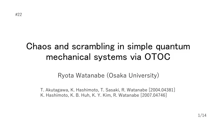
#22 Chaos and scrambling in simple quantum mechanical systems via OTOC Ryota Watanabe (Osaka University) T. Akutagawa, K. Hashimoto, T. Sasaki, R. Watanabe [2004.04381] K. Hashimoto, K. B. Huh, K. Y. Kim, R. Watanabe [2007.04746] 1/14
#22 Chaos and scrambling in simple quantum mechanical systems via OTOC Ryota Watanabe (Osaka University) T. Akutagawa, K. Hashimoto, T. Sasaki, R. Watanabe [2004.04381] K. Hashimoto, K. B. Huh, K. Y. Kim, R. Watanabe [2007.04746] 1/14
Conclusion • The OTOC is more sensitive to quantum chaoticity than the level statistics. • The OTOC detects both chaos and local instability, which may be the information scrambling. 2/14
Contents Introduction • Characteristics of quantum chaos? • Models: coupled/inverted harmonic oscillator OTOC vs Level Statistics • Chaotic model: coupled harmonic oscillator • The OTOC is more sensitive to quantum chaos Chaos vs Scrambling • Microcanonical OTOC • Growth without chaos: inverted harmonic oscillator • Scrambling: thermal OTOC Conclusion & Questions 3/14
Characteristics of quantum chaos? Level Statistics OTOC The repulsion of energy levels The exponential growth of [Larkin, Ovchinnikov `69] [Kitaev `14] Wigner distribution • A bound on chaos [Maldacena, Shenker, Stanford `16] • Does scrambling equal chaos? [Xu, Scaffidi, Cao `19] Simple toy models are being 0 spacing looked for. 4/14
PHYSICAL REVIEW LETTERS VOLUME 52, NUMBER 19 7 MAY 1984 The abscissa is in units of D which time on an IBM 370/168 utilizing gy intervals. thereby almost is all of the core. in the between adjacent levels the average spacing of the analysis of a given In order to perform a statistical interval. Here respective a value energy of k=0. 005 has been chosen. im- parameter spectral sequence it is exceedingly coupling appropriately from a Poisson-type distribution to have a constant An obvious trend portant spacing between average [Fig. (la)] to levels26 the interval since global variations in low-lying energy neighboring energy of the state density mea- in the high-energy distributions can falsify the fluctuation Wigner-type regime [Figs. 1(b) and 1(c)] can be seen. We are able to sures Various procedures considerably. unfolding by a con- into sec- are known to decompose the histograms conveniently a given spectrum approximate 26 27 Here we have Pq(S) function tinuous distribution specified and fluctuations. ular variations by used cubic spline for smoothing the parameter with an appropriate q: of knots to describe number the secular variations S~exp( — P, (S) = PSt+q); (2) level density of the spectrum of H of the integrated n = (1+ q)P, [Eq. (1)] in a given energy A second im- interval. point is the necessity of large data sets in or- portant P = [D- tr [(2+ q)/(1+ q)]]'+q. For der to obtain reasonable measures. fluctuation q =0 P~(S) recovers consider each interval investigated we energy For the Poisson distribution — Pp(S) = (1/D )exp( — q = 1 200 energy limit for a reliable levels as a lower S/D ), for the and Pt(S) = (n S/2D2)exp( — statistical test. mS2/ distribution Wigner of the spacings The distributions between adja- 4D2). It was introduced first by Brody28 in order to cent levels of the unfolded sequence are spectral fit NNS histograms obtained from nuclear spectra. in Fig. 1 for specified ener- as histograms displayed of q displayed in Fig. 1 for The respective values the different have been calculated intervals energy fit. by a least-squares to observed the transition from regularity Having 35 85 E & & Models for a specific Hamiltonian we now vary irregularity Levels 292 50— = 0. 271 the k. Figure in its parameter 2 shows coupling q of the part the variation q parameters with upper Energy values of k [Eq. (1)]. For their energy for different of length 50 we used energy intervals computation of the respective centers are the abscissae whose N I I I I of the curves to the A coupled harmonic oscillator A continuation points. data (U 135 85 E & & more converged require eigenvalues. right would Levels (D 569 q will tend to unity = 0. 508 it is evident that However, as q the value of the coupling the energy param- and/or 50— The curves have been truncated eter k increase. at for low- since the the left-hand side, histograms K charac- exhibit the anomalies intervals lying energy E z of of oscillators teristic harmonic as systems 175 225 E by Berry and Tabor. 2o & & analyzed thoroughly 608 Levels the functional In order to elucidate dependence = 0. 812 • A reduction of Yang-Mills-Higgs theory q on the energy E and the of the Brody parameter k we employ the scaling proper- parameter coupling 50— ty of the classical Hamilton function [Matinyan, Savvidy, T. A. Savvidy `81] q2 jk ), = (1/k) H(1;pt Jk, qt Jk, p2Jk, • Chaotic at high energies (3) FIG. 1. Nearest-neighbor-spacing for ener- histograms where H(k; pt, qt, p2, q2) is the classical [Matinyan, Savvidy, T. A. Savvidy `81] [Haller, Köppel, Cederbaum `84] Hamilton [Eq. (1)] gy levels of the Pullen-Edmonds Hamiltonian to the quantum mechanical with k = 0. 005. The results for three different function corresponding in- energy Hof Eq. (1). It means that the classi- Hamiltonian Brody dis- In each case a best-fitting are shown. tervals on the kE. cal dynamics product depends solely [Eq. (2)] specified by the parameter q is also tribution in Fig. 2(b) the Brody Therefore, we have plotted shown. 1666 An inverted harmonic oscillator • Nonchaotic, but there is an unstable point (nonzero classical Lyapunov) 5/14
Contents Introduction • Characteristics of quantum chaos? • Models: coupled/inverted harmonic oscillator OTOC vs Level Statistics • Chaotic model: coupled harmonic oscillator • The OTOC is more sensitive to quantum chaos Chaos vs Scrambling • Microcanonical OTOC • Growth without chaos: inverted harmonic oscillator • Scrambling: thermal OTOC Conclusion & Questions 6/14
<latexit sha1_base64="6JaxiO2fIrtxgdBxQkYq8nZ3bM=">ACZnichVHLSsNAFD2Nr1ofrYouCmWiqs69YHiqgLl3YB9RSkjitoWkSkrRQiz8guLULVwoi4me48Qdc9A8UlxXcuPA2DYgW9Q4zc+bMPXfOzEiGqlg2Y2PMDA4NDziHfWNjU9M+gNT0xlLr5kyT8u6qps5SbS4qmg8bSu2ynOGycWqpPKsVNnt7mfr3LQUXTuwGwYvVMWypQUWbSJSqVW9oqBEIswJ4L9IOqCENyI64FbHOIOmTUAWHBpuwChEWtTyiYDCIK6BJnElIcfY5TuEjbY2yOGWIxFZoLNMq7Iarbs1LUct0ykqdZOUQYTZE7tjHfbI7tkL+/i1VtOp0fXSoFnqablR9J/Np97/VptnH8pfrTs40SthyvCnk3HKZ7C7mnr5+0OqntZLi5xK7ZK/m/Ym32QDfQ6m/yTYInL+GjD4j+fO5+kFmNRNciG4n1UGzH/QovFrCIZXrvTcSwjzjSdG4Z57hAy/MsTAqzwlwvVfC4mhl8CyH4CeA2imE=</latexit> Chaotic model: Coupled Harmonic Oscillator [Akutagawa, Hashimoto, Sasaki, Watanabe 2004.04381] with 253 energy eigenstates Exponential growth seen in OTOC Chaos not seen in level statistics Exponential growth 30 25 Eigenstates totally symmetric under 𝐷 !" symmetry 20 15 Oscillatory 10 5 0 0 1 2 3 4 5 𝐸 : the average spacing S/D 7/14
Non-Wigner Exponential 4 5 1 0 Wigner Classical growth Oscillatory 2 Chaotic Mixed Regular statistics Level OTOC Quantum 3 The OTOC is more sensitive to chaos [Akutagawa, Hashimoto, Sasaki, Watanabe 2004.04381] E or T ≈ 8/14
Contents Introduction • Characteristics of quantum chaos? • Models: coupled/inverted harmonic oscillator OTOC vs Level Statistics • Chaotic model: coupled harmonic oscillator • The OTOC is more sensitive to quantum chaos Chaos vs Scrambling • Microcanonical OTOC • Growth without chaos: inverted harmonic oscillator • Scrambling: thermal OTOC Conclusion & Questions 9/14
Microcanonical OTOC [Hashimoto, Murata, Yoshii `17] • Energy eigenstates • Thermal OTOC = thermal average of microcanonical OTOC 10/14
Growth without chaos: Inverted Harmonic Oscillator [Hashimoto, Huh, Kim, Watanabe 2007.04746] The potential and the levels Microcanonical OTOC Red: growth is seen V ( x ) Exponential growth 40 4 30 n = 1 n = 5 ln [ c n ( t )] 2 20 n = 9 0 n = 11 10 n = 13 Oscillatory - 2 n = 20 x 0 1 2 3 4 - 10 - 5 0 5 10 t The exponential growth originates from the local instability, not chaos. 11/14
Scrambling: Thermal OTOC [Hashimoto, Huh, Kim, Watanabe 2007.04746] Temperature dependence of Thermal OTOC the Lyapunov exponent Exponential growth 2.2 4 3 2.1 2 2.0 ln [ C T ( t )] T = 1 1 ! "#"$ 1.9 T = 5 0 T = 9 1.8 - 1 T = 30 Oscillatory 1.7 - 2 1.6 0 1 2 3 4 10 20 30 40 50 60 70 80 0 % t is non-vanishing in Semiclassically, is bounded by the classical Lyapunov from below [Xu, Scaffidi, Cao `19]. 12/14
Contents Introduction • Characteristics of quantum chaos? • Models: coupled/inverted harmonic oscillator OTOC vs Level Statistics • Chaotic model: coupled harmonic oscillator • The OTOC is more sensitive to quantum chaos Chaos vs Scrambling • Microcanonical OTOC • Growth without chaos: inverted harmonic oscillator • Scrambling: thermal OTOC Conclusion & Questions 13/14
Conclusion & Questions • The OTOC is more sensitive to quantum chaoticity than the level statistics. • The OTOC detects both chaos and local instability, which may be the information scrambling. Ø Is there any simple quantum mechanical system that saturates the chaos bound? Ø What is actually scrambled? 14/14
Classical chaos in the coupled Harmonic Oscillator [Matinyan, Savvidy, T. A. Savvidy `81] Poincaré sections [Akutagawa, Hashimoto, Sasaki, Watanabe 2004.04381] Chaos (E=20) Regular (E=1) Mixed (E=2) 1 4 1 0.5 2 0.5 0 0 0 -0.5 -2 -0.5 -1 -4 5 -2 0 1 2 -5 -1 -1 -0.5 0 0.5 1 0 𝐹
Recommend
More recommend
Explore More Topics
Stay informed with curated content and fresh updates.

