Causal Regularization for Distributional Robustness and - - PowerPoint PPT Presentation

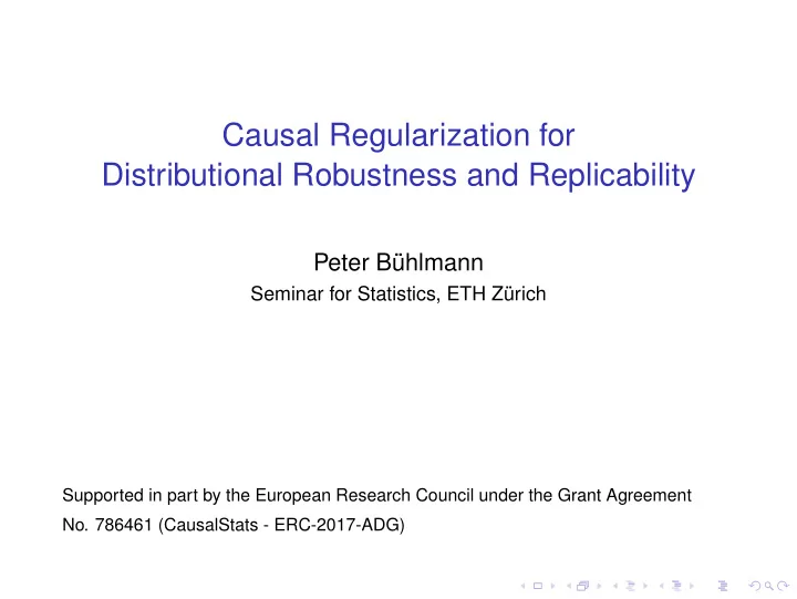
Causal Regularization for Distributional Robustness and Replicability

Peter B¨ uhlmann

Seminar for Statistics, ETH Z¨ urich

Supported in part by the European Research Council under the Grant Agreement

• No. 786461 (CausalStats - ERC-2017-ADG)

Acknowledgments

Dominik Rothenh¨ ausler Stanford University Niklas Pfister ETH Z¨ urich Jonas Peters

• Univ. Copenhagen

Nicolai Meinshausen ETH Z¨ urich

The replicability crisis in science

... scholars have found that the results of many scientific studies are difficult or impossible to replicate (Wikipedia)

John P .A. Ioanidis (School of Medicine, courtesy appoint. Statistics, Stanford) Ioanidis (2005): Why Most Published Research Findings Are False (PLOS Medicine)

• ne among possibly many reasons:

(statistical) methods may not generalize so well...

Single data distribution and accurate inference

say something about generalization to a population from the same distribution as the observed data

Graunt & Petty (1662), Arbuthnot (1710), Bayes (1761), Laplace (1774), Gauss (1795, 1801, 1809), Quetelet (1796-1874),..., Karl Pearson (1857-1936), Fisher (1890-1962), Egon Pearson (1895-1980), Neyman (1894-1981), ...

Bayesian inference, bootstrap, high-dimensional inference, selective inference, ...

Generalization to new data distributions

generalization beyond the population distributions(s) in the data replicability for new data generating distributions setting:

• bserved data from distribution P0

want to say something about new P′ = P0

Generalization to new data distributions

generalization beyond the population distributions(s) in the data replicability for new data generating distributions setting:

• bserved heterogeneous data from distributions Pe (e ∈ E)

E = observed sub-populations want to say something about new Pe′ (e′ / ∈ E) ❀ “some kind of extrapolation” ❀ “some kind of causal thinking” can be useful (as I will try to explain)

see also “transfer learning” from machine learning (cf. Pan and Yang)

GTEx data Genotype-Tissue Expression (GTEx) project a (small) aspect of entire GTEx data: ◮ 13 different tissues, corresponding to E = {1, 2, . . . , 13} ◮ gene expression measurements for 12’948 genes (one of them is the response, the other are covariates) sample size between 300 - 700 ◮ we aim for: prediction for new tissues e′ / ∈ E replication of results on new tissues e′ / ∈ E it’s very noisy and high-dimensional data!

“Causal thinking” we want to generalize/transfer to new situations with new unobserved data generating distributions causality: is giving a prediction (a quantitative answer) to a “what if I do/perturb” question but the perturbation (aka “new situation”) is not observed

many modern applications are faced with such prediction tasks: ◮ genomics: what would be the effect of knocking down (the activity of) a gene on the growth rate of a plant? we want to predict this without any data on such a gene knock-out (e.g. no data for this particular perturbation) ◮ E-commerce: what would be the effect of showing person “XYZ” an advertisement on social media? no data on such an advertisement campaign for “XYZ” or persons being similar to “XYZ” ◮ etc.

Heterogeneity, Robustness and a bit of causality

assume heterogeneous data from different known observed environments or experimental conditions or perturbations or sub-populations e ∈ E: (X e, Y e) ∼ Pe, e ∈ E with response variables Y e and predictor variables X e examples:

• data from 10 different countries
• data from 13 different tissue types in GTEx data

consider “many possible” but mostly non-observed environments/perturbations F ⊃ E

• bserved

examples for F:

• 10 countries and many other than the 10 countries
• 13 different tissue types and many new ones (GTEx example)

problem:

predict Y given X such that the prediction works well

(is “robust”/“replicable”) for “many possible” new environments e ∈ F based on data from much fewer environments from E

trained on designed, known scenarios from E

trained on designed, known scenarios from E new scenario from F!

a pragmatic prediction problem: predict Y given X such that the prediction works well (is “robust”/“replicable”) for “many possible” environments e ∈ F based on data from much fewer environments from E for example with linear models: find argminβ max

e∈F E|Y e − X eβ|2

it is “robustness”

• distributional robust.

a pragmatic prediction problem: predict Y given X such that the prediction works well (is “robust”/“replicable”) for “many possible” environments e ∈ F based on data from much fewer environments from E for example with linear models: find argminβ max

e∈F E|Y e − X eβ|2

it is “robustness”

• distributional robust.

a pragmatic prediction problem: predict Y given X such that the prediction works well (is “robust”/“replicable”) for “many possible” environments e ∈ F based on data from much fewer environments from E for example with linear models: find argminβ max

e∈F E|Y e − X eβ|2

it is “robustness”

• distributional robust.

and causality

Causality and worst case risk

for linear models: in a nutshell for F = {all perturbations not acting on Y directly}, argminβ max

e∈F E|Y e − X eβ|2 = causal parameter = β0

X Y E

β0

that is: causal parameter optimizes worst case loss w.r.t. “very many” unseen (“future”) scenarios

Causality and worst case risk

for linear models: in a nutshell for F = {all perturbations not acting on Y directly}, argminβ max

e∈F E|Y e − X eβ|2 = causal parameter = β0

X Y E

β0

X Y H hidden E

β0

that is: causal parameter optimizes worst case loss w.r.t. “very many” unseen (“future”) scenarios

causal parameter optimizes worst case loss w.r.t. “very many” unseen (“future”) scenarios

no causal graphs or potential outcome models (Neyman, Holland, Rubin, ..., Pearl, Spirtes, ...)

causality and distributional robustness are intrinsically related (Haavelmo, 1943)

Trygve Haavelmo, Nobel Prize in Economics 1989

L(Y e|X e

causal) remains invariant w.r.t. e

causal structure = ⇒ invariance/“robustness”

causal parameter optimizes worst case loss w.r.t. “very many” unseen (“future”) scenarios

no causal graphs or potential outcome models (Neyman, Holland, Rubin, ..., Pearl, Spirtes, ...)

causality and distributional robustness are intrinsically related (Haavelmo, 1943)

Trygve Haavelmo, Nobel Prize in Economics 1989

L(Y e|X e

causal) remains invariant w.r.t. e

causal structure ⇐ = invariance (Peters, PB & Meinshausen, 2016)

causal parameter optimizes worst case loss w.r.t. “very many” unseen (“future”) scenarios causality and distributional robustness are intrinsically related (Haavelmo, 1943)

Trygve Haavelmo, Nobel Prize in Economics 1989

causality ⇐ ⇒ invariance/“robustness” and novel causal regularization allows to exploit this relation

Anchor regression: as a way to formalize the extrapolation from E to F

(Rothenh¨

ausler, Meinshausen, PB & Peters, 2018)

the environments from before, denoted as e: they are now outcomes of a variable A

• anchor

X Y H

hidden

A

β0

?

Anchor regression and causal regularization

(Rothenh¨

ausler, Meinshausen, PB & Peters, 2018)

the environments from before, denoted as e: they are now outcomes of a variable A

• anchor

X Y H

hidden

A

β0

Y ← Xβ0 + εY + Hδ, X ← Aα0 + εX + Hγ,

Instrumental variables regression model (cf. Angrist, Imbens, Lemieux, Newey, Rosenbaum, Rubin,...)

Anchor regression and causal regularization

(Rothenh¨

ausler, Meinshausen, PB & Peters, 2018)

the environments from before, denoted as e: they are now outcomes of a variable A

• anchor

X Y H

hidden

A

β0

A is an “anchor”

source node!

❀ Anchor regression   X Y H   = B   X Y H   + ε + MA

Anchor regression and causal regularization

(Rothenh¨

ausler, Meinshausen, PB & Peters, 2018)

the environments from before, denoted as e: they are now outcomes of a variable A

• anchor

X Y H

hidden

A

β0

A is an “anchor”

source node!

allowing also for feedback loops

❀ Anchor regression   X Y H   = B   X Y H   + ε + MA

allow that A acts on Y and H

❀ there is a fundamental identifiability problem cannot identify β0

this is the price for more realistic assumptions than IV model

... but “Causal Regularization” offers something find a parameter vector β such that the residuals (Y − Xβ) stabilize, have the “same” distribution across perturbations of A = environments/sub-populations we want to encourage orthogonality of residuals with A something like ˜ β = argminβY − Xβ2

2/n + ξAT(Y − Xβ)/n2 2

˜ β = argminβY − Xβ2

2/n + ξAT(Y − Xβ)/n2 2

causal regularization: ˆ β = argminβ(I − ΠA)(Y − Xβ)2

2/n + γΠA(Y − Xβ)2 2/n

ΠA = A(ATA)−1AT

(projection onto column space of A)

◮ for γ = 1: least squares ◮ for 0 ≤ γ < ∞: general causal regularization

˜ β = argminβY − Xβ2

2/n + ξAT(Y − Xβ)/n2 2

causal regularization: ˆ β = argminβ(I − ΠA)(Y − Xβ)2

2/n + γΠA(Y − Xβ)2 2/n + λβ1

ΠA = A(ATA)−1AT

(projection onto column space of A)

◮ for γ = 1: least squares + ℓ1-penalty ◮ for 0 ≤ γ < ∞: general causal regularization + ℓ1-penalty

convex optimization problem

... there is a fundamental identifiability problem... but causal regularization solves for argminβ max

e∈F E|Y e − X eβ|2

for a certain class of shift perturbations F

recap: causal parameter solves for argminβ maxe∈F E|Y e − X eβ|2 for F = “essentially all” perturbations

Model for F: shift perturbations model for observed heterogeneous data (“corresponding to E”)   X Y H   = B   X Y H   + ε + MA model for shift perturbations F (in test data) shift vectors v   X v Y v Hv   = B   X v Y v Hv   + ε + v v ∈ Cγ ⊂ span(M), γ measuring the size of v

i.e. v ∈ Cγ = {v; v = Mu for some u with E[uuT] γE[AAT]}

A fundamental duality theorem (Rothenh¨

ausler, Meinshausen, PB & Peters, 2018)

PA the population projection onto A: PA• = E[•|A]

For any β max

v∈Cγ E[|Y v − X vβ|2] = E

• (Id − PA)(Y − Xβ)
• 2

+ γE

• PA(Y − Xβ)
• 2

≈ (I − ΠA)(Y − Xβ)2

2/n + γΠA(Y − Xβ)2 2/n

• bjective function on data

worst case shift interventions ← → regularization!

in the population case

❀ just regularize! (instead of l.h.s. which is a difficult object)

for any β worst case test error

• max

v∈Cγ E

• Y v − X vβ
• 2

= E

• (Id − PA)(Y − Xβ)
• 2

+ γE

• PA(Y − Xβ)
• 2
• criterion on training population sample

argminβ worst case test error

• max

v∈Cγ E

• Y v − X vβ
• 2

= argminβ E

• (Id − PA)(Y − Xβ)
• 2

+ γE

• PA(Y − Xβ)
• 2
• criterion on training population sample

❀ and “therefore” also finite sample guarantees for predictive stability (i.e. optimizing a worst case risk)

(we have worked out all the details)

distributional robustness ← → causal regularization Adversarial Robustness

machine learning, Generative Networks

e.g. Ian Goodfellow Causality e.g. Judea Pearl

and indeed, one can improve prediction

with causal-type regularization ◮ image classification with CNN (Heinze-Deml and Meinshausen, 2017)

for problems with domain shift: gross improvement over non-regularized standard optimization

◮ causal-robust machine learning

Leon Bouttou et al. since 2013 (Microsoft and now Facebook)

• ther examples:

◮ UCI machine learning and Kaggle datasets ◮ macro-economics (MSc thesis with KOF Swiss Economic Institute) ❀ small (≈ 5%) but persistent gains

Science aims for causal understanding

... but this may be a bit ambitious... causal inference necessarily requires (often untestable) additional assumptions e.g. in anchor regression model: we cannot find/identify the causal (“systems”) parameter β0 X Y H hidden A

β0

Invariance and “diluted causality” by the fundamental duality in anchor regression: γ → ∞ leads to shift invariance of residuals bγ = argminβE

• (Id − PA)(Y − Xβ)
• 2

+ γE

• PA(Y − Xβ)
• 2

) b→∞ = lim

γ→∞ bγ

❀ shift invariance b→∞ is generally not the causal parameter but because of shift invariance: name it “diluted causal”

note: causal = invariance w.r.t. very many perturbations

notions of associations

marginal correlation regression invariance causal*

under faithfulness conditions, the figure is valid (causal* are the causal variables as in e.g. large parts of Dawid, Pearl, Robins, Rubin, ...)

Stabilizing

John W. Tukey (1915 – 2000)

Tukey (1954) “One of the major arguments for regression instead

• f correlation is potential stability. We are very sure

that the correlation cannot remain the same over a wide range of situations, but it is possible that the regression coefficient might. ... We are seeking stability of our coefficients so that we can hope to give them theoretical significance.”

marginal correlation regression invariance causal*

“Diluted causality”: important proteins for cholesterol

Ruedi Aebersold, ETH Z¨ urich

3934 other proteins

which of those are “diluted causal” for cholesterol experiments with mice: 2 environments with fat/low fat diet

high-dimensional regression, total sample size n = 270 Y = cholesterol pathway activity, X = 3934 protein expressions

x-axis: importance w.r.t regression but non-invariant y-axis: importance w.r.t. invariance

0610007P14Rik Acsl3 Acss2 Ceacam1 Cyp51 Dhcr7 Fdft1 Fdps Gpx4 Gstm5 Hsd17b7 Idi1 Mavs Nnt Nsdhl Pmvk Rdh11 Sc4mol Sqle

0.00 0.25 0.50 0.75 1.00 0.00 0.25 0.50 0.75 1.00 selection probability − NSBI(Y) selection probability − SBI(Y)

beyond cholesterol: with transcriptomics and proteomics

not all of the predictive variables from regression lead to invariance!

• ●
• ●
• ●
• ●
• ●
• ●

• ●
• ●
• ●
• ●
• Psmb6

• ●
• ●
• Pdia4

• ●
• ●
• ●
• Gnb2l1

• ●●
• Etfa

• ●
• ●
• Dlst

• ● ●
• Gm5453

• ●
• ●
• ●
• ●
• Eef1b2

• ●
• ●
• ●
• ●
• ●
• ● ●
• ●
• ●
• Acaa1a

• Acaa1b

• ●
• ●
• ●●
• ●
• ●
• Hnrnpa2b1

• ●
• ●
• ●

• ●
• ●
• ● ●●
• ●
• ●
• Ran

• ●
• ●
• ●●
• ●
• ●
• ●
• ●
• ●
• ●
• ●
• ●
• ●
• Txn1

• ●
• ●
• Erg28

• ●
• ● ● ●
• Rdh11

marginal correlation regression invariance causal*

and we actually find promising candidates we “checked” in independent datasets the top hits ❀ has worked “quite nicely” further “validation” with respect to finding known pathways (here for Ribosome pathway)

Ribosome − diet, mRNA

• 0.0

0.2 0.4 corr corr (env) IV (Lasso) Lasso Ridge SRpred SR

pAUC

• − 0.4

− 0.2 0.0 corr corr (env) IV (Lasso) Lasso Ridge SRpred

relative pAUC

Distributional Replicability

The replicability crisis ... scholars have found that the results of many scientific studies are difficult or impossible to replicate (Wikipedia)

more severe issue than just “accurate confidence”, “selective inference”, ...

The “diluted causal” parameter b→∞ is replicable assume ◮ new dataset for replication arises from shift perturbations (as before) ◮ a practically checkable so-called projectability condition

infb E[Y − Xb|A] = 0

consider b→∞ which is estimated from the first dataset b′→∞ which is estimated from the second (new) dataset Then: b→∞ is replicable, i.e., b→∞ = b′→∞

Replicability for b→∞ in GTEx data across tissues ◮ 13 tissues ◮ gene expression measurements for 12’948 genes, sample size between 300 - 700 ◮ Y = expression of a target gene X = expressions of all other genes A = 65 PEER factors (potential confounders) estimation and findings on one tissue ❀ are they replicable on other tissues?

Average replicability for b→∞ in GTEx data across tissues

5 10 15 20 2 4 6 8 10 12 K number of replicable features on a different tissue anchor regression − anchor regression lasso − anchor regression lasso − lasso

x-axis: number K for the top K features y-axis: overlap of the top K ranked variables/features (found by a method on tissue t and on tissue t′ = t)

averaged over all 13 t and averaged over 1000 random choices of a gene as the response

additional information in anchor regression path! the anchor regression path: anchor stability: b0 = b→∞(= bγ ∀γ ≥ 0) checkable! assume: ◮ anchor stability ◮ projectability condition ❀ the least squares parameter b1 is replicable! we can safely use “classical” least squares principle and methods (Lasso/ℓ1-norm regularization, de-biased Lasso, etc.) for transferability to some class of new data generating distributions Pe′ e′ / ∈ E

Replicability for least squares par. in GTEx data across tissues

5 10 15 20 1 2 3 4 K number of replicable features on a different tissue anchor regression − anchor regression lasso − anchor regression lasso − lasso

x-axis: “model size” = K y-axis: how many of the top K ranked associations (found by a method on a tissue t are among the top K on a tissue t′ = t

summed over 12 different tissues t′ = t, averaged over all 13 t and averaged over 1000 random choice of a gene as the response

We can make relevant progress by exploiting invariances/stability

◮ finding more promising proteins and genes: based on high-throughput proteomics ◮ replicable findings across tissues: based on high-throughput transcriptomics ◮ prediction of gene knock-downs (not shown today): based

• n transcriptomics

(Meinshausen, Hauser, Mooij, Peters, Versteeg, and PB, 2016) ◮ large-scale kinetic systems (not shown today): based on metabolomics (Pfister, Bauer and Peters, 2019)

Conclusions

◮ causal regularization is for the population case

(not because of “complexity” in relation to sample size)

❀ distributional robustness and replicability (not claiming to find “truly causal” structure) ◮ the key is to exploit certain invariances ◮ anchor regression (with γ large) justifies instrumental variables regression when IV assumptions are violated ❀ “diluted causality” and invariance of residuals

make heterogeneity or non-stationarity your friend

(rather than your enemy)!

make heterogeneity or non-stationarity your friend

(rather than your enemy)!

Theorem (Rothenh¨

ausler, Meinshausen, PB & Peters, 2018)

assume:

◮ a “causal” compatibility condition on X (weaker than the standard compatibility condition); ◮ (sub-) Gaussian error;

◮ dim(A) ≤ C < ∞ for some C; Then, for Rγ(u) = maxv∈Cγ E|Y v − X vu|2 and any γ ≥ 0: Rγ(ˆ βγ) = min

u Rγ(u)

• ptimal

+OP(sγ

• log(d)/n),

sγ = supp(βγ), βγ = argminβRγ(u) if dim(A) is large: use ℓ∞-norm causal regularization ◮ good for identifiability (lots of heterogeneity) regularization ◮ a statistical price of log(|A|)

Distributionally robust optimization:

(Ben-Tal, El Ghaoui & Nemirovski, 2009; Sinha, Namkoong & Duchi, 2017)

arminβ max

P∈P EP[(Y − Xβ)2]

perturbations are within a class of distributions P = {P; d(P, P0

• emp. distrib.

) ≤ ρ} the “model” is the metric d(., .) and is simply postulated

• ften as Wasserstein distance

metric d(.,.)

Perturbations from distributional robustness

radius rho

learned from data amplified anchor regression robust optimization pre−specified radius perturbations

causal regularization: the class of perturbations is an amplification of the observed and learned heterogeneity from E