c i,j max k,m c k,m 4 Wednesday, 26 Feb. 2020 Machine Learning - PowerPoint PPT Presentation
Uses of Nearest Neighbors } Once we have found the k -nearest neighbors of a point, we can use this information: In and of itself : sometimes we just want to know what 1. those nearest neighbors actually are (items that are similar to a given
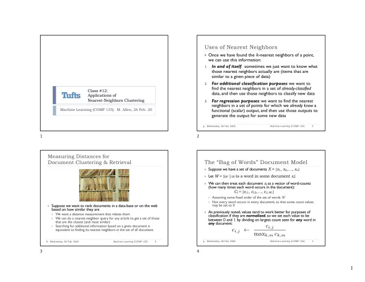
Uses of Nearest Neighbors } Once we have found the k -nearest neighbors of a point, we can use this information: In and of itself : sometimes we just want to know what 1. those nearest neighbors actually are (items that are similar to a given piece of data) For additional classification purposes : we want to 2. find the nearest neighbors in a set of already-classified Class #12: data, and then use those neighbors to classify new data Applications of Nearest-Neighbors Clustering For regression purposes : we want to find the nearest 3. neighbors in a set of points for which we already know a Machine Learning (COMP 135): M. Allen, 26 Feb. 20 functional (scalar) output, and then use those outputs to generate the output for some new data 2 Wednesday, 26 Feb. 2020 Machine Learning (COMP 135) 1 2 Measuring Distances for The “Bag of Words” Document Model Document Clustering & Retrieval } Suppose we have a set of documents X = { x 1 , x 2 ,…, x n } } Let W = { w | w is a word in some document x i } } We can then treat each document x i as a vector of word-counts (how many times each word occurs in the document): C i = { c i, 1 , c i, 2 ,…, c i, | W | } } Assuming some fixed order of the set of words W } Not every word occurs in every document, so that some count values may be set to 0 } Suppose we want to rank documents in a data-base or on the web based on how similar they are } As previously noted, values tend to work better for purposes of } We want a distance measurement that relates them classification if they are normalized , so we set each value to be } We can do a nearest-neighbor query for any article to get a set of those between 0 and 1 by dividing on largest count seen for any word in that are the closest (and most similar) any document: } Searching for additional information based on a given document is c i,j equivalent to finding its nearest neighbors in the set of all document c i,j ← max k,m c k,m 4 Wednesday, 26 Feb. 2020 Machine Learning (COMP 135) 3 Wednesday, 26 Feb. 2020 Machine Learning (COMP 135) 3 4 1
<latexit sha1_base64="9AlSyY3dNL6afTRkAF6okxiuCqU=">ACiHicZVFNa9wEJXdr8T92rTHXIbutmwhbG03kORQCMmlxS62UC8GK0sb0Rky0j2MH41/T/9J5/E63XPbgZkBhG72ZeVoVUhj0/QfHfb8xctXO7ve6zdv370f7X24NKrUjM+ZkpfrajhUuR8jgIlvyo0p9lK8sXq9nzvrj2giV/8b7gi8zus5FKhFW4pHf1hcT6uv8OUHRMhrbKIxoMi4gUrpBCbVBRjpTYgckgUKzOeI0zqSQtR5EW6lLzxC2ybILS3xyKDOq47uYzWcVNBZImLFvo+Q1LYkXBaHdTbEVJNWbOFtk0v1sajsT/zu4CnSdAnY9LHRTz6G/0blUlqzHVguy0bqlEwyVsvKg0vKLula950Frbw2ZYSJW2xy7YVQe4XGFn2YB9XWJ6vGxEXpTIc7aVSUsJqGDjNiRCc4by3iaUaWH7A7uhdkm0fzJQ2piSHMDd5iMTO6tcK4u/yUI7rzUg+H/dp8lOAu+z8Jfh+PTs96KHbJPpEpCcgROSU/yQWZE+bsOt+cY+fE9VzfPXJPtlDX6TkfySDcs0dGBsDG</latexit> Distances between Words Better Measures of Document Similarity We want to emphasize rare words over common ones: } We can now compute the distance function between any } Define word frequency: t(w,x) as the (normalized) count of occurrences of word 1. two documents (here we use the Euclidean): w in document x v c x ( w ) = # times word w occurs in document x | W | u u X d ( x i , x j ) = ( c i,k − c j,k ) 2 t c ? x = max w ∈ W c x ( w ) k =1 t ( w, x ) = c x ( w ) } We could then build a KD-Tree, using the vectors of c ? x words as our dimension values, and query for some set of Define inverse document frequency of word w : 2. most similar documents to any document we start with Total # of | X | documents id ( w ) = log } Problem : word counts turn out to be a lousy metric! 1 + |{ x ∈ X | w ∈ x }| # that contain word w } Common every-day words dominate the counts, making most Use combined measure for each word and document: 3. documents appear quite similar, and making retrieval poor tid ( w, x ) = t ( w, x ) × id ( w ) 6 Wednesday, 26 Feb. 2020 Machine Learning (COMP 135) 5 Wednesday, 26 Feb. 2020 Machine Learning (COMP 135) 5 6 Inverse Document Frequency An Example } The inverse document frequency of word w : } We want to emphasize rare words over common ones: | X | id ( w ) = log | X | 1 + |{ x ∈ X | w ∈ x }| id ( w ) = log } Suppose we have 1,000 documents ( | X | = 1000 ), and the word 1 + |{ x ∈ X | w ∈ x }| the occurs in every single one of them: id ( the ) = log 1000 tid ( w, x ) = t ( w, x ) × id ( w ) 1001 ≈ − 0 . 001442 } Conversely, if the word banana only appears in 10 of them: } id ( w ) goes to 0 as the word w becomes more common id ( banana ) = log 1000 ≈ 6 . 644 } tid ( w,x ) is highest when w occurs often in document x , but 10 is rare overall in the full document set } Thus, when calculating normalized word-counts, banana gets treated as being about 4,600 times more important than the ! } If we threshold id ( w ) to a minimum of 0 (never negative) we then completely ignore words that are in every document 8 Wednesday, 26 Feb. 2020 Machine Learning (COMP 135) 7 Wednesday, 26 Feb. 2020 Machine Learning (COMP 135) 7 8 2
<latexit sha1_base64="RNW3oSmy0/Xtc0SYqhDUtdbRE=">ADC3icnVJLb9NAEF6bVwmPpnDksiIqiqUS2Wml9lKpKheORSJNpWxqbdabdJO1+yO+5Dlf1D+DNygV67c+TesHaPW5IDESLuancf3zc7MJXCgO/ctx79x8fLT2uPXk6bPn6+2NF8dGZrxAVNS6ZMJNVyKhA9AgOQnqeY0nkg+nCzelf7hOdGqOQjXKV8HNZIqaCUbCmcMPZjLqXodjCl+Hcw2/2MTGfNOTEZHGYL/aD4jQnjOoHxYF7oKIuhfhowWHn6L7znfaLzAhLaIzyXM/hSLfLu/Wv1BHcAeUgIi5wUtgb2xJbt3zFXfF+V+kNcIfwEYN9mO3lBVH2O74Pb8SvKoEtdJBtRyF7Z8kUiyLeQJMUmNGga1qnFMNgkletEhmeErZgs54Xk2xwJvWFOGp0vYkgCtrIy5RUE2tkT3KYLo3zkWSZsATtoSZhKDwuXAcSQ0ZyCvrEKZFpYfszOqKQO7Fg2ksoXRFj4vdymytcqZsvFncd/WaxsQ/P3dVeW43wu2e/0PO52Dw7oVa+gVeo26KEC76AC9R0dogJhz7Xxvjs37mf3q/vNvVmGuk6d8xI1xP3xGzHQ8EY=</latexit> Nearest-Neighbor Clustering Image source: Hastie, et al., Elements of Distances between Words for Image Classification Statistical Learning (Springer, 2017) Given the threshold on the inverse document frequency, the distance between two } Spectral Band 1 Spectral Band 2 Spectral Band 3 documents is now proportional to that measure: v | W | u u X d ( x i , x j ) = ( tid ( w k , x i ) − tid ( w k , x j )) 2 t k =1 v | W | u Spectral Band 4 Land Usage Predicted Land Usage u X = ([ t ( w k , x i ) × id ( w k )] − [ t ( w k , x j ) × id ( w k )]) 2 t k =1 v | W | u u X ( id ( w k ) × [ t ( w k , x i ) − t ( w k , x j )]) 2 = t k =1 } The STATLOG project (Michie et al., 1994): given satellite imagery of land, predict its agricultural use for mapping purposes Our KD-T ree can now efficiently find similar documents based upon this metric } Mathematically, words for which frequency id ( w ) = 0 have no effect on the distance } } T raining set: sets of images in 4 spectral bands, with actual use of Obviously, in implementing this we can simply remove those words from word-set W in the first land (7 soil/crop categories) based upon manual survey } place to skip useless clock-cycles… 10 Wednesday, 26 Feb. 2020 Machine Learning (COMP 135) 9 Wednesday, 26 Feb. 2020 Machine Learning (COMP 135) 9 10 Nearest-Neighbor Clustering Image source: Hastie, et al., Elements of Nearest-Neighbor Regression for Image Classification Statistical Learning (Springer, 2017) } Given a data-set of various Spectral Band 1 Spectral Band 2 Spectral Band 3 features of abalone (sex, size, weight, etc.), a regression N N N classifier predicts shellfish age N X N } A training set of Spectral Band 4 Land Usage Predicted Land Usage measurements, with real age N N N determined by counting rings in the abalone shell, is analyzed and grouped into nearest neighbor units } T o predict the usage for a given pixel in a new image: In each band, get value of a pixel and 8 adjacent, for (4 x 9) = 36 features 1. } A predictor for new data is Find the 5 nearest neighbors of that feature-vector in labeled training set 2. generated according to the Assign the land use class of the majority of those 5 neighbors 3. average age value of neighbors } Achieved test error of 9.5% with a very simple algorithm 12 Wednesday, 26 Feb. 2020 Machine Learning (COMP 135) 11 Wednesday, 26 Feb. 2020 Machine Learning (COMP 135) 11 12 3
Nearest-Neighbor Regression Coming Up Next 1-nearest neighbor 5-nearest neighbors } Topics : Support Vector Machines (SVMs) and kernel methods } Readings linked from class schedule page } Assignments : } Project 01: due Monday, 09 March, 5:00 PM } Feature engineering and classification for image data } Midterm Exam: Wednesday, 11 March } Practice exam distributed next week } Review session in class, Monday, 09 March } Office Hours : 237 Halligan } Predictions for 100 points, given regression on shell length and age } Monday, 10:30 AM – Noon } With one-nearest neighbor (left), the result has higher variability and predictions are noisier } Tuesday, 9:00 AM – 1:00 PM } With five-nearest neighbors (right), results are smoothed out over } TA hours can be found on class website multiple data-points 14 Wednesday, 26 Feb. 2020 Machine Learning (COMP 135) 13 Wednesday, 26 Feb. 2020 Machine Learning (COMP 135) 13 14 4
Recommend
More recommend
Explore More Topics
Stay informed with curated content and fresh updates.








![Pr [ X i ] . i = 1 E [ X ] = Pr [ X i ] . i = 1 Proof: One has E [](https://c.sambuz.com/1004042/pr-x-i-i-1-e-x-pr-x-i-i-1-proof-one-has-e-x-s.webp)

