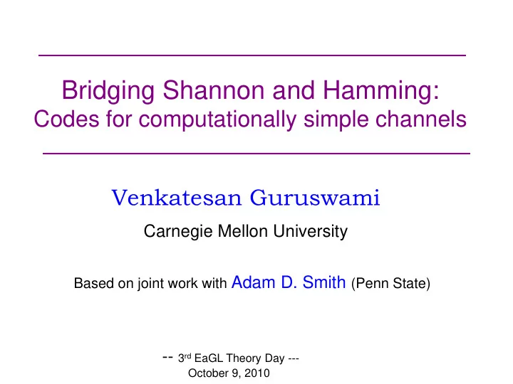
Bridging Shannon and Hamming: Codes for computationally simple - PowerPoint PPT Presentation

Bridging Shannon and Hamming: Codes for computationally simple channels Venkatesan Guruswami Carnegie Mellon University Based on joint work with Adam D. Smith (Penn State) -- 3 rd EaGL Theory Day --- October 9, 2010

Outline • Background & context – Error models, Shannon & Hamming – List decoding • Computationally bounded channels – Previous results (with “setup”) • Our results – Explicit optimal rate codes (for two simple channels) • Proof tools & ideas

Two classic channel models m? m 010100100101 011100001001 Bob Alice Noisy channel • Alice sends n bits • Shannon : Binary symmetric channel BSC p – Flips each bit independently with probability p (error binomially distributed) • Hamming : Worst-case (adversarial) errors ADV p – Channel outputs arbitrary word within distance pn of input Best possible “rate” of reliable information transmission? How many bits can we communicate by sending n bits on channel?

Error-correcting codes (Binary) code: encoding C : {0,1} k  {0,1} n – c = C(m) c • m = message r = c+e • c = codeword Codewords well-separated Rate R = k/n – information per bit of codeword – Want R > 0 as k, n   Idea/hope: codeword c  C can be determined (efficiently) from noisy version r = c + e – e unknown error vector obeying some “noise model”

Shannon capacity limit Hamming ball B(c,pn) Suppose pn bits can get flipped, p  [0,1/2) error fraction pn • c  r = c + e, wt(e)  pn c Decoding region for c  C has volume  2 h(p)n possible r’s • h(p) = - p log 2 p – (1-p) log 2 (1-p ), binary entropy function  Disjoint decoding regions • # codewords  2 n / 2 h(p)n • Rate  1- h(p) Good codes  Good sphere packings

Shannon’s theorem Theorem: There exists a code C : {0,1} Rn  {0,1} n of rate R= 1-h(p)-  such that  m, for e  R Binom(n,p) Pr [ C(m)+e   m’  m B(C(m’),pn) ] ≤ exp( -a  n). Various efficient (polytime encodable/decodable) constructions • Concatenated codes • LDPC codes* • Polar codes i.i.d errors is a strong assumption • eg., errors often bursty… What about worst-case errors? - all we know is wt(e) ≤ pn

Worst-case errors Largest rate of binary code s.t. Hamming balls of radius pn around them are fully disjoint? Answer: Unknown! But it is strictly < 1-h(p) – Rate  0 for p  ¼. – Best known rate (existential) • 1-h(2p) Big price: • for similar rate, can correct only  ½ # errors for worst-case model

A plot rate R BSC p capacity =1-h( p) Approachable efficiently Adv p lower bound = 1-h(2 p ) [G.-V.] p Adv p upper bounds (hand drawn)

Why care about worst-case errors? • As computer scientists, we like to! • “Extraneous” applications of codes – Cryptography, complexity theory (pseudorandomness, hardness amplification, etc.) Communication: Modeling unknown or varying channels – Codes for probabilistic model may fail if stochastic assumptions are wrong • Eg. Concatenated codes for bursty errors – Codes for worst-case errors robust against variety of channels

Bridging Shannon & Hamming I List decoding: Relax decoding goal; recover small list of messages (that includes correct message m) m 1 { LDC(m)+e LDC(m) Deco- m 2 = m m LDC Adv p der ... m L LDC: {0,1} k → {0,1} n is (p,L)-list-decodable if - every y  {0,1} n is within distance pn of  L codewords pn y

List decoding & Shannon capacity Thm [Zyablov- Pinkser’81,Elias’91] : W.h.p., a random code of rate 1-h(p)-  is (p,L)-list-decodable for list size L = 1/   Packing of radius pn Hamming balls covering each point  1/  times [G.-Håstad- Kopparty’10]: Also true for random linear code • Is having a list useful? Yes, for various reasons • better than giving up, • w.h.p. list size 1, • fits the bill perfectly in complexity applications • Versatile primitive (will see in this talk!)

Unfortunately, no constructive result achieving rate  1-h(p) is known for binary list decoding Zyablov radius Optimal trade-off Blokh-Zyablov radius R  1 - h(p) Pre list decoding Constructive: Optimal Tradeoff Zyablov, Blokh-Zyablov: [G.-Rudra ’08,’09 ] Closing this gap Polynomial-based codes + is open Error Fraction concatenation Rate R

Outline • Background & context – Error models, Shannon & Hamming – List decoding • Computationally bounded channels – Previous results (with “setup”) • Our results – Explicit optimal rate codes (for two simple channels) • Proof tools & ideas

Computationally limited channels • Channel models that lie between adversarial channels and specific stochastic assumptions Computationally 010100100101 011100001001 m m Alice Bob “simple” channel • [Lipton’94] : “simple” = simulatable by small circuit – Natural processes may be mercurial, but perhaps not arbitrarily malicious – Eg. O(n 2 ) boolean gates for block length n • Covers models in literature such as AVCs. – studied in [Ding-Gopalan- Lipton’06, Micali -Peikert-Sudan- Wilson’06]

Computationally limited channels Formally: channel class specified by – Complexity of channel – Error parameter p : channel introduces ≤ pn errors w.h.p. Examples: – Polynomial-size: circuits of size n b for known b – Log-space: one-pass circuit using O(log n) bits of memory – Additive channel: XOR with arbitrary oblivious error vector Single code must work for all channels in class

Previous work Need setup assumptions: • [Lipton 1994]: shared secret randomness – Encoder/decoder share random bits s hidden from channel m 010100100101 011100001001 m Alice Bob Noisy channel • [Micali-Peikert-Sudan-Wilson 2006]: public key – Bob, channel have Alice’s public key; only Alice has private key – Alice uses private key to encode

Private codes With shared randomness, don’t even need any computational assumption if we had optimal rate list-decodable codes * [Langberg’04, Smith’07] m 1 ,t 1 t V { m 2 ,t 2 m MAC LDC Dec m V Adv p ... m L ,t L V Idea: Alice authenticates m using s as key • If MAC has forgery probability δ , then Bob fails to uniquely decode m with probability ≤ L δ • MAC tag can have tag & key length O(log n) • O(log n) shared randomness • negligible loss in rate *(which we don’t)

Our Results (Optimal rate) codes with no shared setup 1. Additive errors : efficient, uniquely decodable codes that approach Shannon capacity (1-h(p)) – Previously: only inefficient constructions known via random coding [Cziszar- Narayan’88,’89; Langberg’08] – We also provide a simpler existence proof Formally, explicit randomized code C : {0,1} k x {0,1} r  {0,1} n of rate k/n=1-h(p)-  & efficient decoder Dec such that Decoder doesn’t know encoder’s random bits  m  e, wt(e)  pn, Prob  [ Dec(C(m,  ) + e)= m ] > 1- o(1)

Our Results (Optimal rate) codes with no shared setup 2. Logspace errors : efficient list-decodable code with optimal rate (approaching 1-h(p)) – Previously: no better than uniquely-decodable codes – List decoding = decoder outputs L messages one of which is m w.h.p. ( not all close-by codewords) 3. Polynomial-time errors : efficient list-decodable code with rate  1-h(p), assuming p.r.g.

Why list decoding? Lemma : Unique decoding has rate zero when p > ¼ even for simple bit-fixing channel (which is O(1) space) rate Open : Unique decoding past worst-case errors for p < ¼ for low-space online channels ? p

The ¼ barrier Lemma’s proof idea : • Channel moves codeword c=C(m,  ) towards random codeword c’=C(m’,  ’) , flipping c i with probability ½ when c i  c’ i – constant space – expected fraction of flips  ¼ – Output distribution symmetric w.r.t. inversion of c and c’

Technical Part Additive/oblivious errors Randomized code C : {0,1} k x {0,1} r  {0,1} n of rate k/n=1-h(p)-  & decoding function Dec s.t.  m  e, wt(e)  pn, Prob  [ Dec(C(m,  ) + e)= m ] > 1- o(1)

New existence proof Linear list- decodable code + “additive” MAC ( called A lgebraic M anipulation D etection code , [Cramer-Dodis-Fehr-Padro- Wichs’08] ) m 1 ,  1 ,s 1  V m { AMD Linear List m 2 ,  2 ,s 2  m V m,  ,s code LDC Dec ... e m L ,  L ,s L small random V key Additive error Decoder can disambiguate without knowing  Key point: For fixed e, the additive offsets of the spurious (m i ,  i ,s i ) from (m,  ,s) are fixed. Unlikely these L offsets cause forgery.

Code scrambling: a simple solution with shared randomness π m m additive error REC decoder REC e REC(m)+ π(e) REC(m) π π -1  π -1 (REC(m))+e π -1 (REC(m)) Shared random permutation π of {1,...,n} • Code REC of rate  1-h(p) to correct fraction p random errors [eg. Forney’s concatenated codes] • Encoding : c = π -1 (REC(m)) • Effectively permutes e into random error vector 24

Comment • Similar solution works for adversarial errors Adv p • Shared randomness = ( π,  ) –  acts as one-time pad, making e independent of π m s=(π, Δ) m REC REC decoder REC(m)+ π(e) REC(m) π π -1 π -1 (REC(m)) π -1 (REC(m))+e + Δ + Δ c = π -1 (REC(m))+ Δ Adv p c + e