Branch-Cut-and-Price solver for Vehicle Routing Problems Ruslan - PowerPoint PPT Presentation
Branch-Cut-and-Price solver for Vehicle Routing Problems Ruslan Sadykov 1 , 2 Issam Tahiri 1 , 2 Franois Vanderbeck 2 , 1 Remi Duclos 1 Artur Pessoa 3 Eduardo Uchoa 3 1 2 3 Inria Bordeaux, Universit Bordeaux, Universidade Federal France
Branch-Cut-and-Price solver for Vehicle Routing Problems Ruslan Sadykov 1 , 2 Issam Tahiri 1 , 2 François Vanderbeck 2 , 1 Remi Duclos 1 Artur Pessoa 3 Eduardo Uchoa 3 1 2 3 Inria Bordeaux, Université Bordeaux, Universidade Federal France France Fluminense, Brazil ISMP 2018 Bordeaux, France, July 3 1 / 28
Contents Introduction Web-based solver The algorithm 2 / 28
Modern Branch-Cut-and-Price for Vehicle Routing ◮ Bucket graph-based labelling algorithm for the RCSP pricing [Desrosiers et al., 1983] [Righini and Salani, 2006] [Sadykov et al., 2017] ◮ (Dynamic) partially elementary path ( ng -path) relaxation [Baldacci et al., 2011] [Roberti and Mingozzi, 2014] [Bulhoes et al., 2018] ◮ Automatic dual price smoothing stabilization [Wentges, 1997] [Pessoa et al., 2018b] ◮ Reduced cost fixing of (bucket) arcs in the pricing problem [Ibaraki and Nakamura, 1994] [Irnich et al., 2010] [Sadykov et al., 2017] ◮ Rounded Capacity Cuts [Laporte and Nobert, 1983] [Lysgaard et al., 2004] ◮ Limited-Memory Rank-1 Cuts [Jepsen et al., 2008] [Pecin et al., 2017b] [Pecin et al., 2017c] [Pecin et al., 2017a] ◮ Enumeration of elementary routes [Baldacci et al., 2008] [Contardo and Martinelli, 2014] ◮ Multi-phase strong branching [Røpke, 2012] [Pecin et al., 2017b] 3 / 28
Motivation An expert team needs several months of work to implement a state-of-the-art Branch-Cut-and-Price algorithm Our objective An implementation which may be easily used by researchers 4 / 28
Vehicle Routing Problem Set V of customers, each v ∈ V with demand w v , service time t v and time window [ l v , u v ] . Set M of vehicle types, each m ∈ M with a depot v | V | + m with U m vehicles of capacity W m , with vectors of travel costs c m and travel distances d m . Variants ◮ CVRP (with time windows) ◮ Distance-constrained VRP ◮ Heterogeneous VRP ◮ Multi-depot VRP 6 , 4 , 3 ◮ Site-dependent VRP 5 / 28
Contents Introduction Web-based solver The algorithm 6 / 28
Logging in Address allgo.inria.fr/app/vehiclerouting One needs to sign up (e-mail and password only) and log in. 7 / 28
Running the solver 8 / 28
Parameters roundDistances — whether to round the distances between clients Initial upper bound ◮ By default, jsprit ( github.com/graphhopper/jsprit ) heuristic is used (Ruin-and-Reconstruct Local Search) ◮ jspritMaxIteration — number of iterations in the heuristic (default is 500), ◮ cutOffValue — value specified by the user if given, jsprit heuristic can be turned off (jspritMaxIteration=0) 9 / 28
Supported problems data formats CVRP/DCVRP CVRPLIB format ( vrp.atd-lab.inf.puc-rio.br ) VRPTW [Solomon, 1987] [Gehring and Homberger, 2002] format (total distance objective) MDVRP/SDVRP [Cordeau et al., 1997] format HVRP [Taillard, E. D., 1999] format [Duhamel et al., 2011] format (explicit distances) [Pessoa et al., 2018a] format (CVRPLIB) Other Let us know!!! Other problems Extension to other VRP variants can be considered (contact e-mail is ruslan.sadykov@inria.fr ) 10 / 28
Output of the solver 11 / 28
Example of the branching tree N_1 (56.7s) [8455.08,8662.00] PPN_0 >= 15 PPN_0 <= 14 N_2 (2m20s) N_3 (3m5s) [8658.17,8662.00] [8510.47,8662.00] AggX_0_54_55 >= 1 AggX_0_54_55 <= 0 PPN_1 <= 0 PPN_1 >= 1 N_8 (4m58s) N_9 (5m19s) N_4 (3m11s) N_5 (4m34s) BOUND [8662.00] [8658.90,8662.00] BOUND [8662.00] [8644.29,8662.00] AggX_0_2_57 <= 0 AggX_0_2_57 >= 1 PPN_0 >= 13 PPN_0 <= 12 N_10 (5m39s) N_11 (5m53s) N_6 (4m44s) N_7 (4m45s) BOUND [8662.00] BOUND [8661.81] BOUND [8662.00] BOUND [8662.00] 12 / 28
Remarks ◮ Academic use only ◮ Your instance file is kept on the server ◮ Third party software used: ◮ IBM ILOG Cplex — LP and MIP solver (replacement by Cbc is coming!) ◮ jsprit ( github.com/graphhopper/jsprit ) — heuristic vehicle routing solver ◮ LEMON Graph ibrary ( http://lemon.cs.elte.hu/trac/lemon ) ◮ Boost C++ libraries ( www.boost.org ) ◮ CVRPSEP — RCC separator [Lysgaard et al., 2004] ◮ The solver is in beta version, please report us all issues! 13 / 28
Performance State-of-the-art exact solver for all the problems! Pessoa, A., Sadykov, R., and Uchoa, E. (2018a). Enhanced branch-cut-and-price algorithm for heterogeneous fleet vehicle routing problems. European Journal of Operational Research , 270(2):530–543. Sadykov, R., Uchoa, E., and Pessoa, A. (2017). A bucket graph based labeling algorithm with application to vehicle routing. Cadernos do LOGIS 7, Universidade Federal Fluminense. Remarks ◮ CVRP performance is on pair with [Pecin et al., 2017b] ◮ Performance is very dependent on the initial upper bound 14 / 28
Contents Introduction Web-based solver The algorithm 15 / 28
Set partitioning (master) formulation ◮ R m — set of feasible elementary routes for a type m vehicle ◮ a r v — number of times vertex v appear in route r . ◮ c r — cost of route r ◮ Binary variable λ r = 1 if and only if route r ∈ R m is used by a vehicle of type m � � min c r λ r m ∈ M r ∈ R m � � a r v λ r = 1 , ∀ v ∈ V , m ∈ M r ∈ R m � λ r ≤ U m , ∀ m ∈ M , r ∈ R m λ r ∈ { 0 , 1 } , ∀ r ∈ R m , ∀ m ∈ M . 16 / 28
Pricing sub-problem for a vehicle type m Given dual solution π of the restricted master problem, the pricing problem is � � � c m x r ¯ min c r = ( v , v ′ ) − π v ′ ( v , v ′ ) r ∈ R m v , v ′ ∈ V ′ m i.e. the elementary shortest path problem with capacity and time resources. Labels Each label L = ( v L , ¯ c L , w L , t L , V L ) represents a partial route. It dominates another label L ′ if v L = v L ′ , ¯ c L ≤ ¯ c L ′ , w L ≤ w L ′ , t L ≤ t L ′ , V L ⊆ V L ′ 17 / 28
Partial relaxation of the elementarity : ng -paths [Baldacci et al., 2011] For each vertex v ∈ V , define a memory M v of vertices which “remember” v . If v L �∈ M v , v is removed v L from V L . v M v Sets V L are smaller ⇒ stronger domination Small neighbourhoods (of size ≈ 8-10) produce a tight relaxation of elementarity constraints for most instances. Memories M v are dynamically augmented [Roberti and Mingozzi, 2014] [Bulhoes et al., 2018] Baldacci, R., Mingozzi, A., and Roberti, R. (2011). New route relaxation and pricing strategies for the vehicle routing problem. Operations Research , 59(5):1269–1283. 18 / 28
Non-robust rank-1 cuts [Jepsen et al., 2008] [Pecin et al., 2017b] [Pecin et al., 2017c] [Pecin et al., 2017a] Each cut η ∈ N is obtained by a Chvátal-Gomory rounding of a set C η ⊆ V of set packing constraints using a vector of multipliers ρ η (0 < ρ η v < 1 , v ∈ C η ) ρ η ρ η � � � v a r λ r ≤ � v v m ∈ M r ∈R m v ∈C η v ∈C η ◮ An active cut η ∈ N adds one resource in the RCSP pricing ◮ Limited-memory technique [Pecin et al., 2017b] is critical to reduce the impact on the pricing problem difficulty: for each cut, a memory (on vertices or on arcs) is defined at the separation, making the resource local Pecin, D., Pessoa, A., Poggi, M., and Uchoa, E. (2017b). Improved branch-cut-and-price for capacitated vehicle routing. Mathematical Programming Computation , 9(1):61–100. 19 / 28
Pricing: structure of RCSPP instances ◮ A complete directed graph. ◮ Unrestricted in sign reduced costs on arcs ◮ Two global (capacity and time) resources with non-negative continuous resource consumption ◮ Up to ≈ 500 − 1000 of (more or less) local binary or (small) integer resources ◮ Many different optimal (or near-optimal) solutions. We want to Find a walk minimizing the total reduced cost respecting the resource constrains, as well as many other (up to 1000) different near-optimal feasible walks 20 / 28
Pricing: original graph v = 1 v = 3 source sink v = 2 v = 4 21 / 28
Pricing : the bucket graph [Sadykov et al., 2017] ˜ d 1 bucket v = 1 v = 3 steps ˜ d 2 source sink v = 2 v = 4 u 2 time window l 2 0 capacity W 22 / 28
Pricing : the bucket graph [Sadykov et al., 2017] ˜ d 1 bucket v = 1 v = 3 steps ˜ d 2 source sink v = 2 v = 4 u 2 time window l 2 0 capacity W 22 / 28
Pricing : the bucket graph [Sadykov et al., 2017] ˜ d 1 bucket v = 1 v = 3 steps ˜ d 2 A strongly source sink connected component v = 2 v = 4 u 2 time window l 2 0 capacity W 22 / 28
Bucket graph labeling algorithm [Sadykov et al., 2017] Features: ◮ Bidirectional search + concatenation [Righini and Salani, 2006] ◮ If the bucket graph is acyclic the algorithm is label setting ◮ Otherwise, it becomes label correcting. Buckets in the same strongly connected component are treated together. ◮ The bucket graph structure helps to reduce the number of label dominance checks and speed up concatenation ◮ Arcs in the bucket graph can be fixed by reduced cost, generalizing the fixing schemes in [Ibaraki and Nakamura, 1994] [Irnich et al., 2010] Sadykov, R., Uchoa, E., and Pessoa, A. (2017). A bucket graph based labeling algorithm with application to vehicle routing. Cadernos do LOGIS 7, Universidade Federal Fluminense. 23 / 28
Recommend
More recommend
Explore More Topics
Stay informed with curated content and fresh updates.
