Bootstrap method for misspecified stochastic differential equation - PowerPoint PPT Presentation
Model setting Gaussian quasi-likelihood estimation Bootstrap method for block sum Modified bootstrap method Summary Bootstrap method for misspecified stochastic differential equation models Yuma Uehara The Institute of Statistical
Model setting Gaussian quasi-likelihood estimation Bootstrap method for block sum Modified bootstrap method Summary Bootstrap method for misspecified stochastic differential equation models Yuma Uehara The Institute of Statistical Mathematics Risk and Statistics - 2nd ISM-UUlm Joint Workshop October 8 - October 10, 2019
Model setting Gaussian quasi-likelihood estimation Bootstrap method for block sum Modified bootstrap method Summary Outline Model setting Gaussian quasi-likelihood estimation Diffusion case Pure-jump Lévy driven case Bootstrap method for block sum Pure-jump Lévy driven case Diffusion case Modified bootstrap method Summary
Model setting Gaussian quasi-likelihood estimation Bootstrap method for block sum Modified bootstrap method Summary Model setting Gaussian quasi-likelihood estimation Diffusion case Pure-jump Lévy driven case Bootstrap method for block sum Pure-jump Lévy driven case Diffusion case Modified bootstrap method Summary
Model setting Gaussian quasi-likelihood estimation Bootstrap method for block sum Modified bootstrap method Summary Setting Data-generating model : dX t = A ( X t ) dt + C ( X t − ) dZ t , Statistical model : dX t = a ( X t , α ) dt + c ( X t − , γ ) dZ t • Our estimation target: θ := ( γ, α ) ∈ Θ γ × Θ α := Θ , and the parameter space Θ is a bounded convex space. • The parameter spaces Θ γ and Θ α are subsets of R p γ and R p α , respectively. • The drift coefficients A and a , and the scale coefficients C and c are Lipschitz continuous, and smooth enough, and they and their derivatives are of at most polynomial growth. We further suppose that 1 /c and 1 /C are bounded away from 0.
Model setting Gaussian quasi-likelihood estimation Bootstrap method for block sum Modified bootstrap method Summary Setting (cont’d) • The driving noise Z is a standard Wiener process (hereafter it is sometimes written as w ), or a pure-jump Lévy process with E [ Z t ] = 0 , E [ Z 2 t ] = t , E [ | Z t | q ] < ∞ , and E [ | X t | q ] < ∞ for any q > 0 . Furthermore, we assume that the Blumenthal-Getoor index (BG-index) of Z is smaller than 2, that is, for the Lévy measure ν 0 of Z , � � � | z | γ ν 0 ( dz ) < ∞ β := inf γ ≥ 0 : < 2 . γ | z |≤ 1 • There exists a probability measure π 0 such that for every q > 0 , we can find constants a > 0 and C q > 0 for which sup exp( at ) || P t ( x, · ) − π 0 ( · ) || h q ≤ C q h q ( x ) , t ∈ R + for any x ∈ R where h q ( x ) := 1 + | x | q . • Then we have the ergodic theorem: as T → ∞ , for any polynomial � T p growth function f , 1 � 0 f ( X t ) dt − → f ( x ) π 0 ( dx ) . T
Model setting Gaussian quasi-likelihood estimation Bootstrap method for block sum Modified bootstrap method Summary Setting (cont’d) • Observation: From the solution process X , we suppose that we observe discrete but high-frequency samples ( X t j ) n j =0 under the so-called “rapidly increasing design": t j := t n j = jh n , T n := nh n → ∞ , nh 2 n → 0 . • Model misspecification: Our statistical model is possibly misspecified, i.e., for all θ ∈ Θ , A ( x ) ̸ = a ( x, α ) and C ( x ) ̸ = c ( x, γ ) on the set S , and π 0 ( S ) > 0 . • In general, we cannot avoid the model misspecification. The theory of misspecified models is considered in many papers. For example, Berk (1966), Huber (1967), and White (1984), to mention few. Especially, for stochastic differential equation models, see McKeague (1984), Uchida and Yoshida (2011), Kutoyants (2017), Uehara (2019), and so on. • In this talk, we consider the four cases: the correctly specified diffusion case, the misspecified diffusion case, the correctly specified pure-jump Lévy driven case, and the misspecified pure-jump Lévy driven case.
Model setting Gaussian quasi-likelihood estimation Bootstrap method for block sum Modified bootstrap method Summary Model setting Gaussian quasi-likelihood estimation Diffusion case Pure-jump Lévy driven case Bootstrap method for block sum Pure-jump Lévy driven case Diffusion case Modified bootstrap method Summary
Model setting Gaussian quasi-likelihood estimation Bootstrap method for block sum Modified bootstrap method Summary Gaussian quasi-likelihood estimation • ∆ j X := X t j − X t j − 1 , ∆ j Z := Z t j − Z t j − 1 , f s ( θ ) := f ( X s − , θ ) , f j ( θ ) := f ( X t j , θ ) , ϕ ( x ; µ, Σ) : the density function of the normal distribution whose mean and variance are µ and Σ , respectively. • We define the Gaussian quasi-likelihood estimator ˆ θ n := (ˆ γ n , ˆ α n ) by n � log ϕ (∆ j X ; 0 , h n c 2 γ n = argmax ˆ j − 1 ( γ )) , γ ∈ ¯ Θ γ j =1 n � log ϕ (∆ j X ; h n a j − 1 ( α ) , h n c 2 α n = argmax ˆ j − 1 (ˆ γ n )) . α ∈ ¯ Θ α j =1 • The asymptotic behavior of ˆ θ n is studied in all cases, for instance, see Kessler (1997), Uchida and Yoshida (2011), Masuda (2013), and Uehara (2019).
Model setting Gaussian quasi-likelihood estimation Bootstrap method for block sum Modified bootstrap method Summary Optimal value • We define the optimal value θ ⋆ := ( γ ⋆ , α ⋆ ) by log c 2 ( x, γ ) + C 2 ( x ) � � � γ ⋆ := argmax − π 0 ( dx )(=: G 1 ( γ )) , c 2 ( x, γ ) γ ∈ ¯ Θ γ R − ( A ( x ) − a ( x, α )) 2 � α ⋆ := argmax π 0 ( dx )(=: G 2 ( α )) . c 2 ( x, γ ⋆ ) α ∈ ¯ R Θ α • In the correctly specified case, the optimal value θ ⋆ corresponds to the true value. • We assume the model separability G 1 ( γ ) − G 1 ( γ ⋆ ) ≤ − χ γ | γ − γ ⋆ | 2 , G 2 ( α ) − G 2 ( α ⋆ ) ≤ − χ α | α − α ⋆ | 2 .
Model setting Gaussian quasi-likelihood estimation Bootstrap method for block sum Modified bootstrap method Summary Misspecification bias We illustrate how the misspecification effect appears (since the drift part is almost the same, we look at the scale part). • In the misspecified diffusion case, � T n 1 b ( X s , θ ⋆ ) ds + o p (1) scaled (quasi-)score function = √ T n 0 • In the misspecified pure-jump Lévy driven case, � T n 1 � m ( X s − , θ ⋆ ) ˜ scaled (quasi-)score function = √ T n ¯ N ( ds, dz ) 0 R CLT term � T n 1 b ( X s , θ ⋆ ) ds + o p (1) . + √ T n 0 • ν 0 and ˜ N ( ds, dz ) = N ( ds, dz ) − dsν 0 ( dz ) are the corresponding compensated Poisson random measure, and Lévy measure, respectively.
Model setting Gaussian quasi-likelihood estimation Bootstrap method for block sum Modified bootstrap method Summary Misspecification bias • b is the misspecification bias, and b ( x, θ ⋆ ) π 0 ( dx ) = 0 . � Especially, b ≡ 0 in the correctly specified case. • Although the limit theory for integrals of functional of Markov process is developed in some literature (e.g. Bhattacharya (1982), Komorowski and Walczuk (2012)), its sufficient conditions are difficult to check or the joint asymptotic distribution with the main term is not trivial. • How to correct the misspecification bias?
Model setting Gaussian quasi-likelihood estimation Bootstrap method for block sum Modified bootstrap method Summary Diffusion case (Uchida and Yoshida (2011)) • Let A be the infinitesimal generator of X . • Itô’s formula: for a smooth enough f , � t � f ( X t ) = f ( X 0 ) + 0 A f ( X s ) ds + ∂ x f ( X s ) C ( X s ) dw s . • If there exists a function f solving A f = b , we can transform the bias term: � T n � T n b ( X s , θ ⋆ ) ds = f ( X T n ) − f ( X 0 ) − ∂ x f ( X s ) C ( X s ) dw s . 0 0 • Since the equation A f = b (so-called Poisson equation) is the second order differential equation, the existence of the solution and its regularity is ensured (cf. Pardoux and Veretennikov (2001)).
Model setting Gaussian quasi-likelihood estimation Bootstrap method for block sum Modified bootstrap method Summary Pure-jump Lévy driven case (Uehara (2019)) • We cannot apply the same approach as the diffusion case since the equation A f = b has the integral operator with respect to the Lévy measure. • Instead of A , we consider the extended infinitesimal generator ˜ A of X , and the corresponding extended Poisson equations (cf. Kulik and Veretennikov (2011)). Definition (Kulik and Veretennikov (2011)) We say that a measurable function g : R → R belongs to the domain of the extended generator ˜ A of a càdlàg homogeneous Feller Markov process Y taking values in R if there exists a measurable function b : R → R such that the process � t t ∈ R + , g ( Y t ) − b ( Y s ) ds, 0 is well defined and is a local martingale with respect to the natural filtration of Y and every measure P x ( · ) := P ( ·| Y 0 = x ) , x ∈ R . For EP E such a pair ( g, b ) , we write g ∈ Dom ( ˜ A ) and ˜ A g = b .
Model setting Gaussian quasi-likelihood estimation Bootstrap method for block sum Modified bootstrap method Summary Pure-jump Lévy driven case (cont’d) Uehara (2019), Proposition 3.5 The potential function � ∞ E x [ b ( X t , θ ⋆ )] dt g ( x ) := 0 is the unique solution of ˜ A g = b , and it satisfies that for all p ∈ (1 , ∞ ) p and q = p − 1 , | g ( x ) − g ( y ) | sup | x − y | 1 /p (1 + | x | q + | y | q ) < ∞ . x,y ∈ R ,x ̸ = y • Combined with the martingale representation theorem, we have a similar transformation to the diffusion case.
Recommend
More recommend
Explore More Topics
Stay informed with curated content and fresh updates.
