Blocking in the 2 k Design Blocking may be required because: we - PowerPoint PPT Presentation

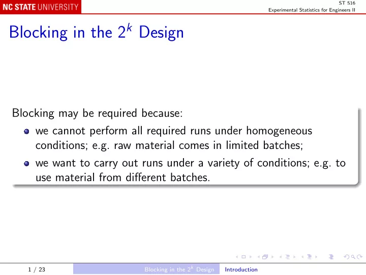
ST 516 Experimental Statistics for Engineers II Blocking in the 2 k Design Blocking may be required because: we cannot perform all required runs under homogeneous conditions; e.g. raw material comes in limited batches; we want to carry out runs under a variety of conditions; e.g. to use material from different batches. Blocking in the 2 k Design 1 / 23 Introduction

ST 516 Experimental Statistics for Engineers II Blocking a Replicated Design If blocks are large enough for 2 k runs, we can carry out each replicate in a single block. E.g. 2 × 2 yield example, in 3 blocks each of 4 runs (yield.txt): summary(aov(Yield ~ Rep + A * B, yield)) Output Df Sum Sq Mean Sq F value Pr(>F) Rep 2 6.500 3.250 0.7852 0.4978348 A 1 208.333 208.333 50.3356 0.0003937 *** B 1 75.000 75.000 18.1208 0.0053397 ** A:B 1 8.333 8.333 2.0134 0.2057101 Residuals 6 24.833 4.139 --- Signif. codes: 0 *** 0.001 ** 0.01 * 0.05 . 0.1 1 Blocking in the 2 k Design 2 / 23 Blocking a Replicated Design

ST 516 Experimental Statistics for Engineers II Analysis as a replicated design This data set was previously analyzed as a replicated design, not blocked: summary(aov(Yield ~ A * B, yield)) Output Df Sum Sq Mean Sq F value Pr(>F) A 1 208.333 208.333 53.1915 8.444e-05 *** B 1 75.000 75.000 19.1489 0.002362 ** A:B 1 8.333 8.333 2.1277 0.182776 Residuals 8 31.333 3.917 --- Signif. codes: 0 *** 0.001 ** 0.01 * 0.05 . 0.1 1 Blocking in the 2 k Design 3 / 23 Blocking a Replicated Design

ST 516 Experimental Statistics for Engineers II Differences 2(= n − 1) degrees of freedom are broken out from “Residuals” into “Rep” (= blocks). Residual mean square changed, and also F-ratios and P-values. Blocking in the 2 k Design 4 / 23 Blocking a Replicated Design

ST 516 Experimental Statistics for Engineers II Confounding If blocks are not large enough for 2 k runs, we must use an incomplete block design . Simplest case: 2 × 2 design in 2 blocks of size 2. Treatment Effect Combination I A B AB Block (1) + - - + 2 a + + - - 1 + - + - 1 b ab + + + + 2 Blocking in the 2 k Design 5 / 23 Confounding

ST 516 Experimental Statistics for Engineers II Note that each block has both levels of A , and also both levels of B , so main effects can be estimated from within-block differences. But the AB interaction is the difference between block averages, and is confounded with blocks. We could also use either the A or B column to assign runs to blocks, but in this case a main effect would be confounded; we usually choose to confound the interaction. Blocking in the 2 k Design 6 / 23 Confounding

ST 516 Experimental Statistics for Engineers II The general 2 k design can be carried out in 2 blocks each of 2 k − 1 runs in the same way: use the signs in the column for the highest-order interaction. Note: runs are sometimes assigned to blocks using a defining contrast L = α 1 x 1 + α 2 x 2 + · · · + α k x k , where: each α i is 1 if factor i is in the interaction to be confounded, and 0 otherwise; x i is 0 for the low level of factor i and 1 for the high level; L is evaluated modulo 2. Blocking in the 2 k Design 7 / 23 Confounding

ST 516 Experimental Statistics for Engineers II Example: a 2 3 design with ABC confounded with blocks Block assignments: Treatment Effect Block Combination I A B AB C AC BC ABC (1) + - - + - + + - 1 a + + - - - - + + 2 + - + - - + - + 2 b ab + + + + - - - - 1 c + - - + + - - + 2 + + - - + + - - 1 ac bc + - + - + - + - 1 + + + + + + + + 2 abc Blocking in the 2 k Design 8 / 23 Confounding

ST 516 Experimental Statistics for Engineers II Terminology: the block containing (1) is the principal block . In this case, the principal block is (1), ab , ac , and bc . These form a group : the product of any pair of elements is another element in the principal block (recall that e.g. a 2 = (1)). You can form the other block by multiplying these by any run not in the principal block, e.g. a or abc . Blocking in the 2 k Design 9 / 23 Confounding

ST 516 Experimental Statistics for Engineers II Example: filtration rate data filtration.txt, 4 factors in 2 blocks: # factors have already been converted from "-","+" to -1, +1 coding filtration$Block <- filtration$A * filtration$B * filtration$C * filtration$D summary(lm(Rate ~ Block + A * B * C * D, filtration)) Note that ABCD cannot be estimated, because it is confounded with blocks. Output Call: lm(formula = Rate ~ Block + A * B * C * D, data = filtration) Residuals: ALL 16 residuals are 0: no residual degrees of freedom! Blocking in the 2 k Design 10 / 23 Confounding

ST 516 Experimental Statistics for Engineers II Output, continued Coefficients: (1 not defined because of singularities) Estimate Std. Error t value Pr(>|t|) (Intercept) 60.0625 NA NA NA Block 0.6875 NA NA NA A 10.8125 NA NA NA B 1.5625 NA NA NA C 4.9375 NA NA NA D 7.3125 NA NA NA A:B 0.0625 NA NA NA A:C -9.0625 NA NA NA B:C 1.1875 NA NA NA A:D 8.3125 NA NA NA B:D -0.1875 NA NA NA C:D -0.5625 NA NA NA A:B:C 0.9375 NA NA NA A:B:D 2.0625 NA NA NA A:C:D -0.8125 NA NA NA B:C:D -1.3125 NA NA NA A:B:C:D NA NA NA NA Blocking in the 2 k Design 11 / 23 Confounding

ST 516 Experimental Statistics for Engineers II Reduced model summary(aov(Rate ~ Block + A + C + D + A * C + A * D, filtration)); Output Df Sum Sq Mean Sq F value Pr(>F) Block 1 7.56 7.56 0.3629 0.5617799 A 1 1870.56 1870.56 89.757 5.600e-06 *** C 1 390.06 390.06 18.717 0.0019155 ** D 1 855.56 855.56 41.053 0.0001242 *** A:C 1 1314.06 1314.06 63.054 2.349e-05 *** A:D 1 1105.56 1105.56 53.049 4.646e-05 *** Residuals 9 187.56 20.84 --- Signif. codes: 0 *** 0.001 ** 0.01 * 0.05 . 0.1 1 Note that all effects in the reduced model can be estimated and tested. Blocking in the 2 k Design 12 / 23 Confounding

ST 516 Experimental Statistics for Engineers II Confounding in More Than 2 Blocks Suppose that blocks hold only 2 k − p runs ⇒ we need 2 p blocks. Choose p effects to be confounded with blocks, where no effect is the product of others. Use the combination of signs in those p columns (or p defining contrasts) to assign runs to blocks. Blocking in the 2 k Design 13 / 23 Confounding

ST 516 Experimental Statistics for Engineers II E.g. a 2 5 design in 4 blocks: we decide to confound ADE and BCE ; Block assignments: Run Block ADE BCE (0) - - Block −− + - Block+ − a b - + Block − + . . . . . . . . . . . . + + Block++ abcde and so on; the four combinations of + and − are used to make four block labels (distinct, but otherwise arbitrary; could be Larry, Moe, Curly, and Shemp). Blocking in the 2 k Design 14 / 23 Confounding

ST 516 Experimental Statistics for Engineers II The 4 blocks are: Block −− : (1) , ad , bc , abcd , abe , ace , cde , bde ; Block+ − : a , d , abc , bcd , be , abde , ce , acde ; Block − +: b , abd , c , acd , ae , de , abce , bcde ; Block++: e , ade , bce , abcde , ab , bd , ac , cd . Note: the 4 blocks will remove 3 degrees of freedom; in addition to ADE and BCE , one other effect must be confounded. It is their product ADE × BCE = ABCDE 2 = ABCD . Note that I , ADE , BCE , and ABCD also form a group. Blocking in the 2 k Design 15 / 23 Confounding

ST 516 Experimental Statistics for Engineers II Replication and Partial Confounding Suppose that a design is replicated and confounded by blocking. If the same confounding structure is used in each replicate, the confounded effects are not estimable; they are said to be completely confounded. If different effects are confounded in each replicate, the design gives some information about all effects; they are said to be partially confounded. Blocking in the 2 k Design 16 / 23 Partial Confounding

ST 516 Experimental Statistics for Engineers II E.g. 2 3 in 2 replicates each in 2 blocks, with ABC confounded with blocks in Rep I, and AB confounded in Rep II (plasma etching tool data): plasmaLongRep1 <- plasmaLong[plasmaLong$Rep == 1,] A <- coded(plasmaLongRep1$A) B <- coded(plasmaLongRep1$B) C <- coded(plasmaLongRep1$C) plasmaLongRep1$Block <- ifelse(A * B * C < 0, 1, 2) plasmaLongRep1 <- plasmaLongRep1[order(plasmaLongRep1$Block),] plasmaLongRep2 <- plasmaLong[plasmaLong$Rep == 2,] A <- coded(plasmaLongRep2$A) B <- coded(plasmaLongRep2$B) plasmaLongRep2$Block <- ifelse(A * B > 0, 1, 2) plasmaLongRep2 <- plasmaLongRep2[order(plasmaLongRep2$Block),] partialConfounding <- rbind(plasmaLongRep1, plasmaLongRep2) partialConfounding$Rep <- factor(partialConfounding$Rep) partialConfounding$Block <- factor(partialConfounding$Block) Blocking in the 2 k Design 17 / 23 Partial Confounding

ST 516 Experimental Statistics for Engineers II partialConfounding A B C Rep Rate id Block 1.1 - - - 1 550 1 1 4.1 + + - 1 642 4 1 6.1 + - + 1 749 6 1 7.1 - + + 1 1075 7 1 2.1 + - - 1 669 2 2 3.1 - + - 1 633 3 2 5.1 - - + 1 1037 5 2 8.1 + + + 1 729 8 2 1.2 - - - 2 604 1 1 4.2 + + - 2 635 4 1 5.2 - - + 2 1052 5 1 8.2 + + + 2 860 8 1 2.2 + - - 2 650 2 2 3.2 - + - 2 601 3 2 6.2 + - + 2 868 6 2 7.2 - + + 2 1063 7 2 Blocking in the 2 k Design 18 / 23 Partial Confounding