Bj ork Chapter (3rd edition) 23 : Short rate models; generalities. - PowerPoint PPT Presentation

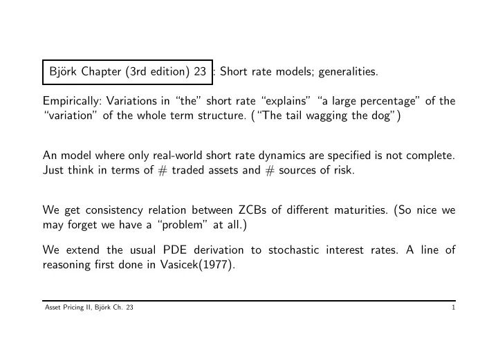
Bj¨ ork Chapter (3rd edition) 23 : Short rate models; generalities. Empirically: Variations in “the” short rate “explains” “a large percentage” of the “variation” of the whole term structure. (“The tail wagging the dog”) An model where only real-world short rate dynamics are specified is not complete. Just think in terms of # traded assets and # sources of risk. We get consistency relation between ZCBs of different maturities. (So nice we may forget we have a “problem” at all.) We extend the usual PDE derivation to stochastic interest rates. A line of reasoning first done in Vasicek(1977). Asset Pricing II, Bj¨ ork Ch. 23 1

Look (first) at the case where dr ( t ) = µ ( t, r ( t )) dt + σ ( t, r ( t )) dW P ( t ) where µ and σ are functions and W P is a 1-dimensional Brownian motion under the real-world probability measure P . So r is Markov wrt. its own filtration. Suppose all kinds of ZCB exist. The “formal” equation � � �� � T P ( t ; T ) = E Q exp r ( u ) du − t t makes us conjecture that P ( t ; T ) = F ( t, r ( t ); T ) Asset Pricing II, Bj¨ ork Ch. 23 2

for some smooth function F (of 3 variables.) Hide T -dependence in a superscript and use Ito to get F T = F T t + µF T r + 1 2 σ 2 F T dF T dt + σF T rr r dW P ( t ) F T F T � �� � � �� � := α T := σ T Now make a self-financing portfolio with a T -ZCB and an S -ZCB. V is the value process and ( u T , u S ) relative portfolio weights. From Chapter 6 we have dF T dF S dV = u T F T + u S F S V ( u T α T + u S α S ) dt + ( u T σ T + u S σ S ) dW P ( t ) = Asset Pricing II, Bj¨ ork Ch. 23 3

By construction we must have u T + u S = 1 , but still 1 degree of freedom. A clever choice is u T σ T + u S σ S = 0 . The dW P -term vanishes, we get − σ S u T = σ T − σ S (symmetric in S ), and α S σ T − α T σ S dV = dt. σ T − σ S V � �� � must = r ( t ) otherwise arbitrage Asset Pricing II, Bj¨ ork Ch. 23 4

Rewriting α S − r ( t ) = α T − r ( t ) σ S σ T LHS doesn’t depend on T , RHS doesn’t depend on S ⇒ the ratio is independent of maturity: α S − r ( t ) := λ ( r ( t ); t ) . σ S λ : “market price of risk”; interpretation as excess expected return relative to volatility. Has to be exogenously specified. Usually: Postulate form that gives same structure under P and Q — a subtlety that people may be obtuse about. Asset Pricing II, Bj¨ ork Ch. 23 5

Substitute back and get the term structure PDE: r + 1 F T t + ( µ − λσ ) F T 2 σ 2 F T rr = rF T and F T ( T ; r ) = 1 This may be Feynman-Kac represented and we may change measure: � � �� � T F ( t, r ( t ); T ) = E Q exp r ( s ) ds − t where dr ( s ) = ( µ − λσ ) ds + σdW Q ( s ) Note: Clearly P ( t ; T ) /β ( t ) is a Q -martingale. Asset Pricing II, Bj¨ ork Ch. 23 6

Writing � � dW P + α T − r ( t ) dP ( t ; T ) P ( t ; T ) = α T ( t ; T ) dt + σ T ( t, T ) dW P = r ( t ) dt + σ T ( t, T ) dt σ T � �� � = dW Q , by Girsanov shows that pieces fit. We’re still not very concrete. Asset Pricing II, Bj¨ ork Ch. 23 7