Binar y data and logistic regression G E N E R AL IZE D L IN E AR - PowerPoint PPT Presentation

Binar y data and logistic regression G E N E R AL IZE D L IN E AR MOD E L S IN P YTH ON Ita Ciro v ic Done v Data Science Cons u ltant

Binar y response data T w o - class response → 0,1 E x amples : Credit scoring → "Default"/"Non-Default" Passing a test → "Pass"/"Fail" Fra u d detection → "Fraud"/"No-Fraud" Choice of a prod u ct → "Product ABC"/"Product XYZ" GENERALIZED LINEAR MODELS IN PYTHON

Binar y data UNGROUPED GROUPED Single e v ent M u ltiple e v ents Flip one coin Flip m u ltiple coins N u mber of s u ccesses in a gi v en n n u mber T w o of possible o u tcomes : 0/1 Bernoulli ( p ) or of trials Binomial ( n , p ) Binomial ( n = 1, p ) GENERALIZED LINEAR MODELS IN PYTHON

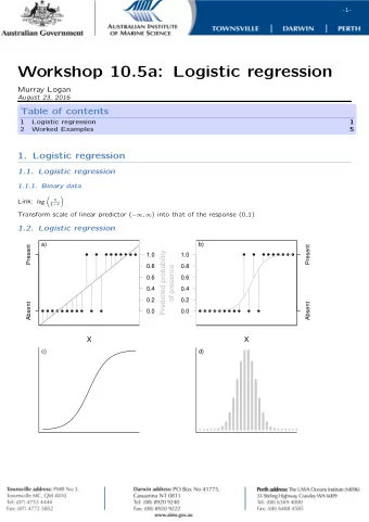
Logistic f u nction GENERALIZED LINEAR MODELS IN PYTHON

Logistic f u nction Test o u tcome : PASS = 1 or FAIL = 0 Want to model P ( y = 1) = β + β x 0 1 1 P (Pass) = β + β × Hours of study 0 1 GENERALIZED LINEAR MODELS IN PYTHON

Logistic f u nction Test o u tcome : PASS = 1 or FAIL = 0 Want to model P ( y = 1) = β + β x 0 1 1 P (Pass) = β + β × Hours of study 0 1 Use logistic f u nction 1 f ( z ) = (1+exp(− z )) GENERALIZED LINEAR MODELS IN PYTHON

Odds and odds ratio event occuring ODDS = event NOT occuring odds 1 ODDS RATIO = odds 2 GENERALIZED LINEAR MODELS IN PYTHON

Odds e x ample 4 games Odds are 3 to 1 GENERALIZED LINEAR MODELS IN PYTHON

Odds and probabilities odds ≠ probability probability odds = 1 − probability odds probability = 1 − odds GENERALIZED LINEAR MODELS IN PYTHON

From probabilit y model to logistic regression Step 3. Appl y logistic f u nction → INVERSE - Step 1. Probabilit y model E ( y ) = μ = P ( y = 1) = β + β x LOGIT 0 1 1 exp( β + β x ) 1 = 0 1 1 μ = 1+exp(−( β + β x )) 1+exp( β + β x ) 0 1 1 0 1 1 1 1 − μ = 1+exp( β + β x ) 0 1 1 Step 2. Logistic f u nction 1 f ( z ) = (1+exp(− z )) GENERALIZED LINEAR MODELS IN PYTHON

From probabilit y model to logistic regression Probabilit y → odds μ ODDS = = exp ( β + β x ) 0 1 1 1 − μ Log transformation → LOGISTIC REGRESSION μ LOGIT ( μ ) = log ( ) = β + β x 0 1 1 1 − μ GENERALIZED LINEAR MODELS IN PYTHON

Logistic regression in P y thon F u nction - glm() model_GLM = glm(formula = 'y ~ x', data = my_data, family = sm.families.Binomial()a).fit Inp u t y = [0,1,1,0,...] y = ['No','Yes','Yes',...] y = ['Fail','Pass','Pass',...] GENERALIZED LINEAR MODELS IN PYTHON

Let ' s practice ! G E N E R AL IZE D L IN E AR MOD E L S IN P YTH ON

Interpreting coefficients G E N E R AL IZE D L IN E AR MOD E L S IN P YTH ON Ita Ciro v ic Done v Data Science Cons u ltant

Model coefficients GENERALIZED LINEAR MODELS IN PYTHON

Coefficient beta β > 0 → ascending c u r v e β < 0 → descending c u r v e GENERALIZED LINEAR MODELS IN PYTHON

Linear v s logistic LINEAR MODEL LOGIT MODEL glm('y ~ weight', glm('y ~ weight', data = crab, data = crab, family = sm.families.Gaussian()) family = sm.families.Binomial()) μ = −0.14 + 0.32 ∗ weight log ( odds ) = −3.69 + 1.8 ∗ weight For e v er y one -u nit increase in w eight For e v er y one -u nit increase in w eight estimated probability increases b y 0.32 log(odds) increase b y 1.8 GENERALIZED LINEAR MODELS IN PYTHON

Log odds interpretation Logistic model μ log ( ) = β + β x 0 1 1 1 − μ Increase x b y one -u nit μ log ( ) = β + β ( x + 1) 0 1 1 1 − μ GENERALIZED LINEAR MODELS IN PYTHON

Log odds interpretation Logistic model μ log ( ) = β + β x 0 1 1 1 − μ Increase x b y one -u nit μ log ( ) = β + β ( x + 1) = β + β x + β 0 1 1 0 1 1 1 1 − μ Take the e x ponential μ ( ) = exp( β + β x )exp( β ) 0 1 1 1 1 − μ Concl u sion → the odds are m u ltiplied b y exp( β ) 1 GENERALIZED LINEAR MODELS IN PYTHON

Log odds interpretation Crab model y ~ weight μ log ( ) = −3.6947 + 1.815 ∗ weight 1 − μ The odds of satellite crab m u ltipl y b y exp(1.815) = 6.14 for a u nit increase in w eight GENERALIZED LINEAR MODELS IN PYTHON

Log odds interpretation Crab model y ~ weight μ log ( ) = −3.6947 + 1.8151 ∗ weight 1 − μ The odds of satellite crab m u ltipl y b y exp(1.8151) = 6.14 for a u nit increase in w eight The intercept coe � cient of −3.6947 denotes the baseline log odds exp(−3.6947) = 0.0248 are the odds w hen weight = 0 . GENERALIZED LINEAR MODELS IN PYTHON

Probabilit y v s logistic fit GENERALIZED LINEAR MODELS IN PYTHON

Probabilit y v s logistic fit GENERALIZED LINEAR MODELS IN PYTHON

Probabilit y v s logistic fit slope → β × μ (1 − μ ) GENERALIZED LINEAR MODELS IN PYTHON

Probabilit y v s logistic fit slope → β × μ (1 − μ ) GENERALIZED LINEAR MODELS IN PYTHON

Comp u te change in estimated probabilit y # Choose x (weight) and extract model coefficients x = 1.5 intercept, slope = model_GLM.params # Compute estimated probability est_prob = np.exp(intercept + slope * x)/(1 + np.exp(intercept + slope * x)) 0.2744 # Compute incremental change in estimated probability given x ic_prob = slope * est_prob * (1 - est_prob) 0.3614 GENERALIZED LINEAR MODELS IN PYTHON

Rate of change in probabilit y for e v er y x logit = −3.6947 + 1.8151 ∗ weight GENERALIZED LINEAR MODELS IN PYTHON

Let ' s practice ! G E N E R AL IZE D L IN E AR MOD E L S IN P YTH ON

Interpreting model inference G E N E R AL IZE D L IN E AR MOD E L S IN P YTH ON Ita Ciro v ic Done v Data Science Cons u ltant

Estimation of beta coefficient Ma x im u m likelihood estimation ( MLE ) ^ β Estimated coe � cient , log - likelihood takes on the ma x im u m v al u e GENERALIZED LINEAR MODELS IN PYTHON

Estimation of beta coefficient Iterati v el y re w eighted least sq u ares ( IRLS ) GENERALIZED LINEAR MODELS IN PYTHON

Significance testing GENERALIZED LINEAR MODELS IN PYTHON

Standard error ( SE ) Fla � er peak Sharper peak → Location of ma x im u m harder to de � ne → Location of ma x im u m more clearl y → Larger SE de � ned → Smaller SE GENERALIZED LINEAR MODELS IN PYTHON

Comp u tation of the standard error # Extract variance-covariance matrix Variance - co v ariance matri x print(model_GLM.cov_params()) Intercept weight Intercept 0.774762 -0.325087 weight -0.325087 0.141903 # Compute standard error for weight std_error = np.sqrt(0.141903) 0.3767 GENERALIZED LINEAR MODELS IN PYTHON

Significance testing z- statistic E x ample : horseshoe crab model ^ z = / SE y ~ weight β z large ⇒ coe � cient ≠ 0 ⇒ v ariable z = 1.8151/0.377 = 4.819 signi � cant R u le of th u mb : c u t - o � v al u e of 2 GENERALIZED LINEAR MODELS IN PYTHON

Confidence inter v als for beta Uncertaint y of the estimates 95% con � dence inter v als for β [ lower , upper ] ^ ^ [ − 1.96 × SE , + 1.96 × SE ] β β GENERALIZED LINEAR MODELS IN PYTHON

Comp u ting confidence inter v als E x ample : horseshoe crab model coef std err ---------------------------------- Intercept -3.6947 0.880 weight 1.8151 0.377 [1.8151 − 1.96 × 0.377, 1.8151 + 1.96 × 0.377] [1.07618, 2.55402] GENERALIZED LINEAR MODELS IN PYTHON

E x tract confidence inter v als print(model_GLM.conf_int()) 0 1 Intercept -5.419897 -1.969555 weight 1.076826 2.553463 GENERALIZED LINEAR MODELS IN PYTHON

E x tract confidence inter v als print(model_GLM.conf_int()) lower 1 Intercept -5.419897 -1.969555 weight 1.076826 2.553463 GENERALIZED LINEAR MODELS IN PYTHON

E x tract confidence inter v als print(model_GLM.conf_int()) 0 upper Intercept -5.419897 -1.969555 weight 1.076826 2.553463 GENERALIZED LINEAR MODELS IN PYTHON

Confidence inter v als for odds 1. E x tract con � dence inter v als for β 2. E x ponentiate endpoints print(np.exp(model_GLM.conf_int())) 0 1 Intercept 0.004428 0.139519 weight 2.935348 12.851533 GENERALIZED LINEAR MODELS IN PYTHON

Let ' s practice ! G E N E R AL IZE D L IN E AR MOD E L S IN P YTH ON

Comp u ting and describing predictions G E N E R AL IZE D L IN E AR MOD E L S IN P YTH ON Ita Ciro v ic Done v Data Science Cons u ltant

Comp u ting predictions A � er obtaining model � t 1. Fi � ed v al u es for original x v al u es GENERALIZED LINEAR MODELS IN PYTHON

Comp u ting predictions A � er obtaining model � t 1. � � ed v al u es for original x v al u es 2. Ne w v al u es of x for predicted v al u es GENERALIZED LINEAR MODELS IN PYTHON

Comp u ting predictions Horseshoe crab model y ~ weight exp(−3.6947 + 1.8151 × weight ) μ = 1 + exp(−3.6947 + 1.8151 × weight ) Ne w meas u rement : weight = 2.85 exp(−3.6947 + 1.8151 × 2.85) μ = = 0.814 1 + exp(−3.6947 + 1.8151 × 2.85) GENERALIZED LINEAR MODELS IN PYTHON

Predictions in P y thon Comp u te model predictions for dataset new_data # Compute model predictions model_GLM.predict(exog = new_data) GENERALIZED LINEAR MODELS IN PYTHON

From probabilities to classes GENERALIZED LINEAR MODELS IN PYTHON