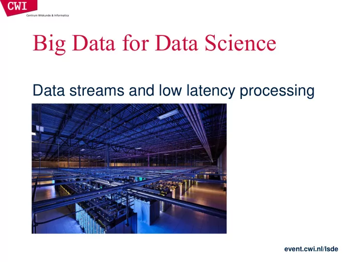
Big Data for Data Science Data streams and low latency processing - PowerPoint PPT Presentation

Big Data for Data Science Data streams and low latency processing event.cwi.nl/lsde

DATA STREAM BASICS event.cwi.nl/lsde2015 event.cwi.nl/lsde

What is a data stream? • Large data volume, likely structured, arriving at a very high rate – Potentially high enough that the machine cannot keep up with it • Not (only) what you see on youtube – Data streams can have structure and semantics, they’re not only audio or video • Definition (Golab and Ozsu, 2003) – A data stream is a real-time, continuous, ordered (implicitly by arrival time of explicitly by timestamp) sequence of items. It is impossible to control the order in which items arrive, nor it is feasible to locally store a stream in its entirety. event.cwi.nl/lsde2015 event.cwi.nl/lsde

Why do we need a data stream? • Online, real-time processing • Potential objectives – Event detection and reaction – Fast and potentially approximate online aggregation and analytics at different granularities • Various applications – Network management, telecommunications Sensor networks, real-time facilities monitoring – Load balancing in distributed systems – Stock monitoring, finance, fraud detection – Online data mining (click stream analysis) event.cwi.nl/lsde2015 event.cwi.nl/lsde

Example uses • Network management and configuration – Typical setup: IP sessions going through a router – Large amounts of data (300GB/day, 75k records/second sampled every 100 measurements) – Typical queries • What are the most frequent source-destination pairings per router? • How many different source-destination pairings were seen by router 1 but not by router 2 during the last hour (day, week, month)? • Stock monitoring – Typical setup: stream of price and sales volume – Monitoring events to support trading decisions – Typical queries • Notify when some stock goes up by at least 5% • Notify when the price of XYZ is above some threshold and the price of its competitors is below than its 10 day moving average event.cwi.nl/lsde2015 event.cwi.nl/lsde

Structure of a data stream • Infinite sequence of items (elements) • One item: structured information, i.e., tuple or object • Same structure for all items in a stream • Timestamping – Explicit: date/time field in data – Implicit: timestamp given when items arrive • Representation of time – Physical: date/time – Logical: integer sequence number event.cwi.nl/lsde2015 event.cwi.nl/lsde

Database management vs. data stream management queries DSMS data feeds DBMS DSMS data streams queries • Data stream management system (DSMS) at multiple observation points – Voluminous streams-in, reduced streams-out • Database management system (DBMS) – Outputs of data stream management system can be treated as data feeds to database event.cwi.nl/lsde2015 event.cwi.nl/lsde

DBMS vs. DSMS • DBMS • DSMS – Model: persistent relations – Model: transient relations – Relation: tuple set/bag – Relation: tuple sequence – Data update: modifications – Data update: appends – Query: transient – Query: persistent – Query answer: exact – Query answer: approximate – Query evaluation: arbitrary – Query evaluation: one pass – Query plan: fixed – Query plan: adaptive event.cwi.nl/lsde2015 event.cwi.nl/lsde

Windows • Mechanism for extracting a finite relation from an infinite stream • Various window proposals for restricting processing scope – Windows based on ordering attributes (e.g., time) – Windows based on item (record) counts – Windows based on explicit markers (e.g., punctuations) signifying beginning and end – Variants (e.g., some semantic partitioning constraint) event.cwi.nl/lsde2015 event.cwi.nl/lsde

Ordering attribute based windows • Assumes the existence of an attribute that defines the order of stream elements/records (e.g., time) • Let T be the window length (size) expressed in units of the ordering attribute (e.g., T may be a time window) sliding window t 2 ’ t 3 ’ t 4 ’ t 1 t 2 t 3 t 4 t 1 ' t i ’ – t i = T t 3 tumbling window t 1 t 2 t i+1 – t i = T event.cwi.nl/lsde2015 event.cwi.nl/lsde

Count-based windows • Window of size N elements (sliding, tumbling) over the stream • Problematic with non-unique timestamps associated with stream elements • Ties broken arbitrarily may lead to non-deterministic output • Potentially unpredictable with respect to fluctuating input rates – But dual of time based windows for constant arrival rates – Arrival rate λ elements/time-unit, time-based window of length T , count- based window of size N ; N = λT t 2 ’ t 3 ’ t 4 ’ t 1 t 2 t 3 t 1 ' event.cwi.nl/lsde2015 event.cwi.nl/lsde

Punctuation-based windows • Application-inserted “end -of- processing” – Each next data item identifies “beginning -of- processing” • Enables data item-dependent variable length windows – Examples: a stream of auctions, an interval of monitored activity • Utility in data processing: limit the scope of operations relative to the stream • Potentially problematic if windows grow too large – Or even too small: too many punctuations event.cwi.nl/lsde2015 event.cwi.nl/lsde

Putting it all together: architecting a DSMS storage query monitor working storage input query output monitor summary processor buffer storage static query storage repository streaming streaming inputs outputs user DSMS queries event.cwi.nl/lsde2015 event.cwi.nl/lsde

STREAM MINING event.cwi.nl/lsde2015 event.cwi.nl/lsde

Data stream mining • Numerous applications – Identify events and take responsive action in real time – Identify correlations in a stream and reconfigure system • Mining query streams: Google wants to know what queries are more frequent today than yesterday • Mining click streams: Yahoo wants to know which of its pages are getting an unusual number of hits in the past hour • Big brother – Who calls whom? – Who accesses which web pages? – Who buys what where? – All those questions answered in real time • We will focus on frequent pattern mining event.cwi.nl/lsde2015 event.cwi.nl/lsde

Frequent pattern mining • Frequent pattern mining refers to finding patterns that occur more frequently than a pre-specified threshold value – Patterns refer to items, itemsets, or sequences – Threshold refers to the percentage of the pattern occurrences to the total number of transactions • Termed as support • Finding frequent patterns is the first step for association rules – A → B : A implies B • Many metrics have been proposed for measuring how strong an association rule is – Most commonly used metric: confidence – Confidence refers to the probability that set B exists given that A already exists in a transaction • confidence( A → B ) = support( A ∧ B ) / support( A ) event.cwi.nl/lsde2015 event.cwi.nl/lsde

Frequent pattern mining in data streams • Frequent pattern mining over data streams differs from conventional one – Cannot afford multiple passes • Minimised requirements in terms of memory • Trade off between storage, complexity, and accuracy • You only get one look • Frequent items (also known as heavy hitters) and itemsets are usually the final output • Effectively a counting problem – We will focus on two algorithms: lossy counting and sticky sampling event.cwi.nl/lsde2015 event.cwi.nl/lsde

The problem in more detail • Problem statement – Identify all items whose current frequency exceeds some support threshold s ( e.g., 0.1%) event.cwi.nl/lsde2015 event.cwi.nl/lsde

Lossy counting in action • Divide the incoming stream into windows event.cwi.nl/lsde2015 event.cwi.nl/lsde

First window comes in • At window boundary, adjust counters event.cwi.nl/lsde2015 event.cwi.nl/lsde

Next window comes in Frequenc y Frequency Counts Counts + Next Window second window frequency counts frequency counts • At window boundary, adjust counters event.cwi.nl/lsde2015 event.cwi.nl/lsde

Lossy counting algorithm • Deterministic technique; user supplies two parameters – Support s ; error ε • Simple data structure, maintaining triplets of data items e , their associated frequencies f , and the maximum possible error ∆ in f : ( e , f , ∆ ) • The stream is conceptually divided into buckets of width w = 1/ ε – Each bucket labelled by a value N/w where N starts from 1 and increases by 1 • For each incoming item, the data structure is checked – If an entry exists, increment frequency – Otherwise , add new entry with ∆ = b current − 1 where b current is the current bucket label • When switching to a new bucket, all entries with f + ∆ < b current are released event.cwi.nl/lsde2015 event.cwi.nl/lsde

Lossy counting observations • How much do we undercount? – If current size of stream is N – ...and window size is 1/ ε – ... then frequency error ≤ number of windows, i .e. , εN • Empirical rule of thumb: set ε = 10% of support s – Example: given a support frequency s = 1%, – …then set error frequency ε = 0.1% • Output is elements with counter values exceeding sN − εN • Guarantees – Frequencies are underestimated by at most εN – No false negatives – False positives have true frequency at least sN − εN • In the worst case, it has been proven that we need 1/ ε × log ( εN ) counters event.cwi.nl/lsde2015 event.cwi.nl/lsde

Sticky Sampling event.cwi.nl/lsde2015 event.cwi.nl/lsde