Beating the random assignment for constraint satisfaction problems - PowerPoint PPT Presentation

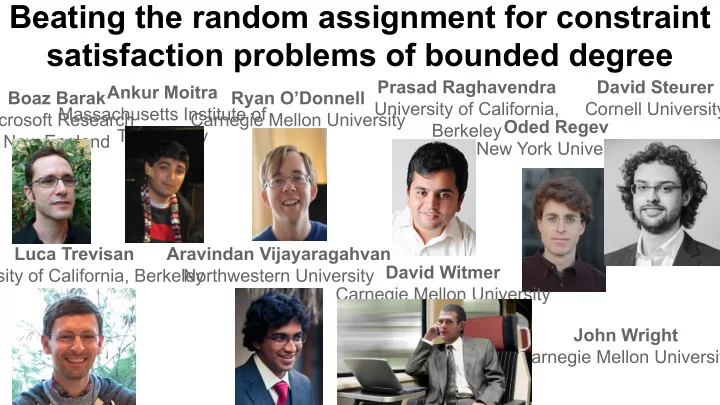
Beating the random assignment for constraint satisfaction problems of bounded degree Prasad Raghavendra David Steurer Ankur Moitra Boaz Barak Ryan O’Donnell University of California, Cornell University Massachusetts Institute of Microsoft Research Carnegie Mellon University Berkeley Oded Regev Technology New England New York University Luca Trevisan Aravindan Vijayaragahvan Northwestern University David Witmer University of California, Berkeley Carnegie Mellon University John Wright Carnegie Mellon University

3XOR x 1 x 3 x 5 = 1 x 10 x 16 x 3 = -1 x 61 x 100 x 2 = 1 ... x 47 x 11 x 98 = -1 x 8 x 2 x 1 = -1

3XOR Q: How many equations can we satisfy? x 1 x 3 x 5 = 1 x 10 x 16 x 3 = -1 x 61 x 100 x 2 = 1 ... x 47 x 11 x 98 = -1 x 8 x 2 x 1 = -1

3XOR Q: How many equations can we satisfy? x 1 x 3 x 5 = 1 Random satisfies ½ on average. x 10 x 16 x 3 = -1 x 61 x 100 x 2 = 1 ... x 47 x 11 x 98 = -1 x 8 x 2 x 1 = -1

3XOR Q: How many equations can we satisfy? x 1 x 3 x 5 = 1 Random satisfies ½ on average. x 10 x 16 x 3 = -1 Q: Can we do better? x 61 x 100 x 2 = 1 ... x 47 x 11 x 98 = -1 x 8 x 2 x 1 = -1

3XOR Q: How many equations can we satisfy? x 1 x 3 x 5 = 1 Random satisfies ½ on average. x 10 x 16 x 3 = -1 Q: Can we do better? x 61 x 100 x 2 = 1 [Håstad 97] : No , not even when ... instance is (1-ε)-satisfiable. x 47 x 11 x 98 = -1 x 8 x 2 x 1 = -1

3XOR Q: How many equations can we satisfy? x 1 x 3 x 5 = 1 Random satisfies ½ on average. x 10 x 16 x 3 = -1 Q: Can we do better? x 61 x 100 x 2 = 1 [Håstad 97] : No , not even when ... instance is (1-ε)-satisfiable. x 47 x 11 x 98 = -1 The end. x 8 x 2 x 1 = -1

There’s more to the story...

There’s more to the story... [HV04] : Can satisfy ½ + Ω( m -1/2 )-fraction if only m equations.

There’s more to the story... [HV04] : Can satisfy ½ + Ω( m -1/2 )-fraction if only m equations. [KN08] : Can satisfy ½ + Ω( ε (log( n )/ n ) ½ )-fraction if only n variables if OPT = ½ + ε .

There’s more to the story... [HV04] : Can satisfy ½ + Ω( m -1/2 )-fraction if only m equations. [KN08] : Can satisfy ½ + Ω( ε (log( n )/ n ) ½ )-fraction if only n variables if OPT = ½ + ε . This work : What if instance is degree bounded , i.e. every variable appears in ≤ D clauses?

Degree bounded schmegree bounded....

Degree bounded schmegree bounded.... Degree-bounded instances exist in the wild e.g. : PCP Theorem spits out 5 -bounded 3Sat instances.

Degree bounded schmegree bounded.... Degree-bounded instances exist in the wild e.g. : PCP Theorem spits out 5 -bounded 3Sat instances. [Hås00] : Can approximate any degree bounded CSP to factor μ + O(1/ D ).

Degree bounded schmegree bounded.... Degree-bounded instances exist in the wild e.g. : PCP Theorem spits out 5 -bounded 3Sat instances. [Hås00] : Can approximate any degree bounded CSP to factor μ + O(1/ D ). [Tre01] : For 3XOR, can’t approximate better than ½ + O( D -1/2 ).

Our inspiration [FG14] introduce Q uantum A pproximate O ptimization A lgorithm

Our inspiration [FG14] introduce Q uantum A pproximate O ptimization A lgorithm [FGG15] : Given 3Lin instance, QAOA satisfies

Our inspiration [FG14] introduce Q uantum A pproximate O ptimization A lgorithm [FGG15] : Given 3Lin instance, QAOA satisfies - ½ + Ω( D -3/4 )-fraction of eqn’s if D -degree bounded

Our inspiration [FG14] introduce Q uantum A pproximate O ptimization A lgorithm [FGG15] : Given 3Lin instance, QAOA satisfies - ½ + Ω( D -3/4 )-fraction of eqn’s if D -degree bounded - ½ + Ω( D -1/2 )-fraction if also triangle-free

Our inspiration [FG14] introduce Q uantum A pproximate O ptimization A lgorithm [FGG15] : Given 3Lin instance, QAOA satisfies - ½ + Ω( D -3/4 )-fraction of eqn’s if D -degree bounded - ½ + Ω( D -1/2 )-fraction if also triangle-free

Main theorem Given a D -degree bounded k -Lin instance, can find (in poly-time) an assignment x such that | val ( x ) - ½| ≥ Ω k ( D -1/2 ).

Main theorem Given a D -degree bounded k -Lin instance, can find (in poly-time) an assignment x such that | val ( x ) - ½| ≥ Ω k ( D -1/2 ).

Main theorem Given a D -degree bounded k -Lin instance, can find (in poly-time) an assignment x such that | val ( x ) - ½| ≥ Ω k ( D -1/2 ). If k is odd , then for x or its negation - x , val (± x ) ≥ ½ + Ω k ( D -1/2 ).

Main theorem Given a D -degree bounded k -Lin instance, can find (in poly-time) an assignment x such that | val ( x ) - ½| ≥ Ω k ( D -1/2 ). If k is odd , then for x or its negation - x , val (± x ) ≥ ½ + Ω k ( D -1/2 ). (and this is easily shown to be tight)

Somewhere in Sweden... Independently of us, Johan Håstad proved the same result.

Somewhere in Sweden... Independently of us, Johan Håstad proved the same result. After our work... [FGG] : for 3Lin, the QAOA algo finds x s.t. val ( x ) ≥ ½ + Ω( D -1/2 log( D ) -1 ).

Let’s do the proof for k = 3.

Step 1: Decoupling x 1 x 3 x 5 = 1 x 10 x 16 x 3 = -1 ... x 47 x 11 x 98 = -1

Step 1: Decoupling x 1 x 3 x 5 = 1 x 10 x 16 x 3 = -1 (transformation) ... x 47 x 11 x 98 = -1

Step 1: Decoupling y 6 z 4 z 32 = 1 x 1 x 3 x 5 = 1 y 3 z 2 z 34 = 1 x 10 x 16 x 3 = -1 (transformation) ... ... y 86 z 71 z 23 = -1 x 47 x 11 x 98 = -1

Step 1: Decoupling y 6 z 4 z 32 = 1 x 1 x 3 x 5 = 1 y 3 z 2 z 34 = 1 x 10 x 16 x 3 = -1 (transformation) ... ... y 86 z 71 z 23 = -1 x 47 x 11 x 98 = -1 [KN08] : can assume WOLOG that instance is decoupled

Step 2: The algorithm y 6 z 4 z 32 = 1 y 3 z 2 z 34 = 1 ... y 86 z 71 z 23 = -1

Step 2: The algorithm y 6 z 4 z 32 = 1 1.) Assign the z i ’s to be iid y 3 z 2 z 34 = 1 random bits. ... y 86 z 71 z 23 = -1

Step 2: The algorithm y 6 z 4 z 32 = 1 1.) Assign the z i ’s to be iid y 3 z 2 z 34 = 1 random bits. ... 2.) Pick each y i to satisfy the y 86 z 71 z 23 = -1 maximum number of equations.

Step 2: The algorithm y 6 (-1) = 1 1.) Assign the z i ’s to be iid y 3 z 2 z 34 = 1 random bits. ... 2.) Pick each y i to satisfy the y 86 z 71 z 23 = -1 maximum number of equations.

Step 2: The algorithm y 6 (-1) = 1 1.) Assign the z i ’s to be iid y 3 (1) = 1 random bits. ... 2.) Pick each y i to satisfy the y 86 z 71 z 23 = -1 maximum number of equations.

Step 2: The algorithm y 6 (-1) = 1 1.) Assign the z i ’s to be iid y 3 (1) = 1 random bits. ... 2.) Pick each y i to satisfy the y 86 (1) = -1 maximum number of equations.

Given a set of m equations y i1 z i2 z i3 = b i

Given a set of m equations y i1 z i2 z i3 = b i total # of satisfied equations is ∑ i (½ + ½ b i y i1 z i2 z i3 )

Given a set of m equations y i1 z i2 z i3 = b i total # of satisfied equations is ∑ i (½ + ½ b i y i1 z i2 z i3 ) = m /2 + ½ ∑ i b i y i1 z i2 z i3

Given a set of m equations y i1 z i2 z i3 = b i total # of satisfied equations is ∑ i (½ + ½ b i y i1 z i2 z i3 ) = m /2 + ½ ∑ i b i y i1 z i2 z i3 Goal: want this to be mD -1/2 larger than m /2

Given a set of m equations y i1 z i2 z i3 = b i total # of satisfied equations is ∑ i (½ + ½ b i y i1 z i2 z i3 ) = m /2 + ½ ∑ i b i y i1 z i2 z i3 Goal: want this to be mD -1/2 larger than m /2 ⇒ want ∑ i b i y i1 z i2 z i3 ≥ mD -1/2

Rewrite ∑ i b i y i1 z i2 z i3

Rewrite ∑ i b i y i1 z i2 z i3 = ∑ j y j ∙G j ( z )

Rewrite ∑ i b i y i1 z i2 z i3 = ∑ j y j ∙G j ( z ) After picking z ’s, best y j = sgn (G j ( z )).

Rewrite ∑ i b i y i1 z i2 z i3 = ∑ j y j ∙G j ( z ) After picking z ’s, best y j = sgn (G j ( z )). ∴ can always achieve ∑ j |G j ( z )|.

Rewrite ∑ i b i y i1 z i2 z i3 = ∑ j y j ∙G j ( z ) After picking z ’s, best y j = sgn (G j ( z )). ∴ can always achieve ∑ j |G j ( z )|. G j ( z ) is a quadratic with deg ( y j ) many ±1 terms

Rewrite ∑ i b i y i1 z i2 z i3 = ∑ j y j ∙G j ( z ) After picking z ’s, best y j = sgn (G j ( z )). ∴ can always achieve ∑ j |G j ( z )|. G j ( z ) is a quadratic with deg ( y j ) many ±1 terms ∴ Var (G j ( z )) = deg ( y j )

Rewrite ∑ i b i y i1 z i2 z i3 = ∑ j y j ∙G j ( z ) After picking z ’s, best y j = sgn (G j ( z )). ∴ can always achieve ∑ j |G j ( z )|. G j ( z ) is a quadratic with deg ( y j ) many ±1 terms ∴ Var (G j ( z )) = deg ( y j ) ∴ E z |G j ( z )| ≥ deg ( y j ) 1/2

Rewrite ∑ i b i y i1 z i2 z i3 = ∑ j y j ∙G j ( z ) After picking z ’s, best y j = sgn (G j ( z )). ∴ can always achieve ∑ j |G j ( z )|. G j ( z ) is a quadratic with deg ( y j ) many ±1 terms ∴ Var (G j ( z )) = deg ( y j ) ∴ E z |G j ( z )| ≥ deg ( y j ) 1/2 ∴ E z ∑ j |G j ( z )| ≥ ∑ j deg ( y j ) 1/2

Rewrite ∑ i b i y i1 z i2 z i3 = ∑ j y j ∙G j ( z ) After picking z ’s, best y j = sgn (G j ( z )). ∴ can always achieve ∑ j |G j ( z )|. G j ( z ) is a quadratic with deg ( y j ) many ±1 terms ∴ Var (G j ( z )) = deg ( y j ) ∴ E z |G j ( z )| ≥ deg ( y j ) 1/2 ∴ E z ∑ j |G j ( z )| ≥ ∑ j deg ( y j ) 1/2 ≥ ∑ j deg ( y j )/ D 1/2