Bayesian nonparametric estimation for quantum homodyne tomography - PowerPoint PPT Presentation
Bayesian nonparametric estimation for quantum homodyne tomography Zacharie Naulet (CEA Saclay and Paris-Dauphine University) Joint work with: ric Barat (CEA Saclay) Judith Rousseau (Paris-Dauphine University) TT. Truong (Cergy-Pontoise
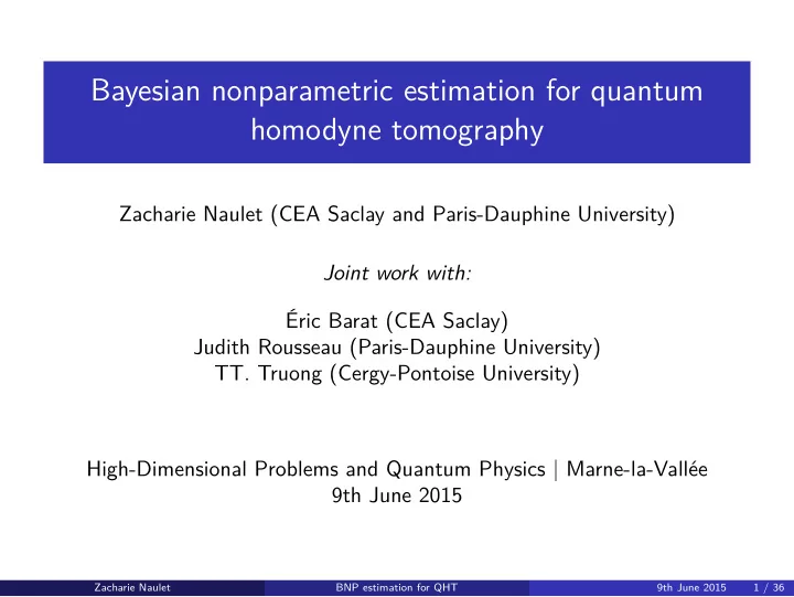
Bayesian nonparametric estimation for quantum homodyne tomography Zacharie Naulet (CEA Saclay and Paris-Dauphine University) Joint work with: Éric Barat (CEA Saclay) Judith Rousseau (Paris-Dauphine University) TT. Truong (Cergy-Pontoise University) High-Dimensional Problems and Quantum Physics | Marne-la-Vallée 9th June 2015 Zacharie Naulet BNP estimation for QHT 9th June 2015 1 / 36
Outline 1 Quantum Homodyne Tomography Quantum Mechanics : Short introduction Quantum Homodyne Tomography Canonical examples of quantum states 2 BNP estimate Mixtures models Square integrable representations and coherent states Completely random measures Summary and sampling Simulation results 3 Asymptotics results ? 4 Conclusion Zacharie Naulet BNP estimation for QHT 9th June 2015 1 / 36
Outline 1 Quantum Homodyne Tomography Quantum Mechanics : Short introduction Quantum Homodyne Tomography Canonical examples of quantum states 2 BNP estimate Mixtures models Square integrable representations and coherent states Completely random measures Summary and sampling Simulation results 3 Asymptotics results ? 4 Conclusion Zacharie Naulet BNP estimation for QHT 9th June 2015 1 / 36
QM : Short introduction A1 With every quantum system is associated an infinite-dimensional separable Hilbert space H over C , with inner product �· , ·� , the space of states . Zacharie Naulet BNP estimation for QHT 9th June 2015 2 / 36
QM : Short introduction A1 With every quantum system is associated an infinite-dimensional separable Hilbert space H over C , with inner product �· , ·� , the space of states . A2 The set of observables A of a quantum system consists of all self-adjoint operators on H . Zacharie Naulet BNP estimation for QHT 9th June 2015 2 / 36
QM : Short introduction A1 With every quantum system is associated an infinite-dimensional separable Hilbert space H over C , with inner product �· , ·� , the space of states . A2 The set of observables A of a quantum system consists of all self-adjoint operators on H . A3 The set of pure states S of a quantum system are projection operators P onto one-dimensional subspaces of H , with Tr P = 1. For ψ ∈ H with � ψ � = 1, we write P ψ : H → H the projection operator (density matrix) onto the linear span of ψ . Zacharie Naulet BNP estimation for QHT 9th June 2015 2 / 36
QM : Short introduction A1 With every quantum system is associated an infinite-dimensional separable Hilbert space H over C , with inner product �· , ·� , the space of states . A2 The set of observables A of a quantum system consists of all self-adjoint operators on H . A3 The set of pure states S of a quantum system are projection operators P onto one-dimensional subspaces of H , with Tr P = 1. For ψ ∈ H with � ψ � = 1, we write P ψ : H → H the projection operator (density matrix) onto the linear span of ψ . A4 A measurement is a mapping A × S ∋ ( A , P ) �→ µ A ∈ P ( R ). Zacharie Naulet BNP estimation for QHT 9th June 2015 2 / 36
QM : Short introduction A1 With every quantum system is associated an infinite-dimensional separable Hilbert space H over C , with inner product �· , ·� , the space of states . A2 The set of observables A of a quantum system consists of all self-adjoint operators on H . A3 The set of pure states S of a quantum system are projection operators P onto one-dimensional subspaces of H , with Tr P = 1. For ψ ∈ H with � ψ � = 1, we write P ψ : H → H the projection operator (density matrix) onto the linear span of ψ . A4 A measurement is a mapping A × S ∋ ( A , P ) �→ µ A ∈ P ( R ). µ A is given by the Born-Von Neumann formula : µ A ( E ) := Tr P A ( E ) P ψ = � P A ( E ) ψ, ψ � , E ∈ B ( R ) , where P A is a positive operator-valued measure which precise definition is stated in Von Neumann’s Spectral Theorem . µ A ( E ) is the probability that the measurement of the observable A on the system in state P ψ lies in E ∈ B ( R ). Zacharie Naulet BNP estimation for QHT 9th June 2015 2 / 36
QM : Simultaneous measurements Definition Self-adjoint operators A and B commute if the corresponding POVM P A and P B satisfy P A ( E 1 ) P B ( E 2 ) = P B ( E 2 ) P A ( E 1 ) for all E 1 , E 2 ∈ B ( R ) . Zacharie Naulet BNP estimation for QHT 9th June 2015 3 / 36
QM : Simultaneous measurements Definition Self-adjoint operators A and B commute if the corresponding POVM P A and P B satisfy P A ( E 1 ) P B ( E 2 ) = P B ( E 2 ) P A ( E 1 ) for all E 1 , E 2 ∈ B ( R ) . A5 Observables A and B can be measured simultaneously if and only if they commute. Zacharie Naulet BNP estimation for QHT 9th June 2015 3 / 36
QM : Simultaneous measurements Definition Self-adjoint operators A and B commute if the corresponding POVM P A and P B satisfy P A ( E 1 ) P B ( E 2 ) = P B ( E 2 ) P A ( E 1 ) for all E 1 , E 2 ∈ B ( R ) . A5 Observables A and B can be measured simultaneously if and only if they commute. Otherwise, we have the celebrated Heisenberg’s uncertainty relations : Theorem Let A , B ∈ A and ψ ∈ D( A ) ∩ D( B ) with A ψ, B ψ ∈ D( A ) ∩ D( B ) . Then, ψ ( B ) ≥ 1 σ 2 ψ ( A ) σ 2 4 � i ( AB − BA ) ψ, ψ � 2 . Zacharie Naulet BNP estimation for QHT 9th June 2015 3 / 36
QM : Simultaneous measurements Definition Self-adjoint operators A and B commute if the corresponding POVM P A and P B satisfy P A ( E 1 ) P B ( E 2 ) = P B ( E 2 ) P A ( E 1 ) for all E 1 , E 2 ∈ B ( R ) . A5 Observables A and B can be measured simultaneously if and only if they commute. Otherwise, we have the celebrated Heisenberg’s uncertainty relations : Theorem Let A , B ∈ A and ψ ∈ D( A ) ∩ D( B ) with A ψ, B ψ ∈ D( A ) ∩ D( B ) . Then, ψ ( B ) ≥ 1 σ 2 ψ ( A ) σ 2 4 � i ( AB − BA ) ψ, ψ � 2 . = ⇒ If A and B don’t commute, there is no joint distribution associated with the measurement of A , B . Example : position Q and momentum P . Zacharie Naulet BNP estimation for QHT 9th June 2015 3 / 36
The Wigner transform Definition Wigner transform Let ψ ∈ L 2 ( R ) with � ψ � 2 = 1, then the Wigner transform W : L 2 ( R ) → L 2 ( R 2 ) is defined as � � � � � W ( ψ )( q , p ) := 1 q + y q − y e − ipy dy , ( q , p ) ∈ R 2 ψ ψ 2 2 π R Zacharie Naulet BNP estimation for QHT 9th June 2015 4 / 36
The Wigner transform Definition Wigner transform Let ψ ∈ L 2 ( R ) with � ψ � 2 = 1, then the Wigner transform W : L 2 ( R ) → L 2 ( R 2 ) is defined as � � � � � W ( ψ )( q , p ) := 1 q + y q − y e − ipy dy , ( q , p ) ∈ R 2 ψ ψ 2 2 π R Properties of the Wigner transform 1 Real valued. � 2 Total energy : R 2 W ( ψ )( q , p ) dqdp = 1. � R W ( ψ )( p , q ) dp = | ψ ( q ) | 2 (proba. density) 3 Marginals : � ψ ( p ) | 2 (proba. density) R W ( ψ )( p , q ) dq = | � 4 Marginals : 5 Isometry : � W ( ψ 1 ) , W ( ψ 2 ) � L 2 ( R 2 ) = � ψ 1 , ψ 2 � L 2 ( R ) Zacharie Naulet BNP estimation for QHT 9th June 2015 4 / 36
The Wigner transform (continued) Properties of the Wigner transform (continued) From the isometry property, if ψ and ϕ are orthogonal, � R 2 W ( ψ )( q , p ) W ( ϕ )( q , p ) dqdp = 0 . = ⇒ There exists locally negative Wigner transforms, and W ( ψ ) can’t be a joint probability density. Zacharie Naulet BNP estimation for QHT 9th June 2015 5 / 36
Outline 1 Quantum Homodyne Tomography Quantum Mechanics : Short introduction Quantum Homodyne Tomography Canonical examples of quantum states 2 BNP estimate Mixtures models Square integrable representations and coherent states Completely random measures Summary and sampling Simulation results 3 Asymptotics results ? 4 Conclusion Zacharie Naulet BNP estimation for QHT 9th June 2015 5 / 36
Quantum Homodyne Tomography Goal : Measuring the quantum state of light. Observables of interest are self-adjoint operators on L 2 ( R ) : 1 P : the magnetic field, P ψ ( x ) = − i ψ ′ ( x ). 2 Q : the electric field, Q ψ ( x ) = x ψ ( x ). 3 ( H = P 2 + Q 2 : the total energy of the electromagnetic field) Zacharie Naulet BNP estimation for QHT 9th June 2015 6 / 36
Quantum Homodyne Tomography Goal : Measuring the quantum state of light. Observables of interest are self-adjoint operators on L 2 ( R ) : 1 P : the magnetic field, P ψ ( x ) = − i ψ ′ ( x ). 2 Q : the electric field, Q ψ ( x ) = x ψ ( x ). 3 ( H = P 2 + Q 2 : the total energy of the electromagnetic field) Obviously PQ � = QP thus we can’t measure simultaneously observables P and Q . But, we can measure the quadrature observables X φ = cos( φ ) Q + sin( φ ) P on n quantum systems in the same state P ψ . 1 We get iid data ( X 1 , φ 1 ) , . . . , ( X n , φ n ) with distribution P ψ on R × [0 , π ]. 2 We aim at estimating P ψ (or equivalently ψ ∈ L 2 ( R )) from the data. Zacharie Naulet BNP estimation for QHT 9th June 2015 6 / 36
QHT : Experimental setup Distribution of X | φ We have iid data ( X 1 , φ 1 ) , . . . , ( X n , φ n ) coming from the measurement of the observables X φ on n quantum systems in the same state P ψ . The distribution of X | φ has density (wrt Lebesgue measure on R ) g ψ ( x | φ ) = R ( W ( ψ ))( x , φ ) � := W ( ψ )( x cos φ − ξ sin φ, x sin φ + ξ cos φ ) d ξ, R Source : Quantum information where R ( W ( ψ )) is the Radon transform of W ( ψ ). technology, a homodyne tomogra- phy tutorial. http://www.iqst.ca/ quantech/homotomo.php . Zacharie Naulet BNP estimation for QHT 9th June 2015 7 / 36
Recommend
More recommend
Explore More Topics
Stay informed with curated content and fresh updates.
