Bayesian inference for discretely observed diffusion processes - PowerPoint PPT Presentation
Bayesian inference for discretely observed diffusion processes Moritz Schauer with Frank van der Meulen and Harry van Zanten Delft University of Technology, University of Amsterdam Van Dantzig Seminar 1 / 25 Estimating parameters of a
Bayesian inference for discretely observed diffusion processes Moritz Schauer with Frank van der Meulen and Harry van Zanten Delft University of Technology, University of Amsterdam Van Dantzig Seminar 1 / 25
Estimating parameters of a discretely observed diffusion process Diffusion process X d X t = b θ ( t, X t ) d t + σ θ ( t, X t ) d W t , X 0 = u, with transition densities p ( s, x ; t, y ) Discrete observations X t i = x i , 0 = t 0 < t 1 < · · · < t n . ◮ Bayesian estimate for parameter θ with prior π 0 ( θ ) . ◮ Likelihood is intractable (product of transition densities) ◮ Continuous time likelihood known in closed form (Girsanov’s theorem) 2 / 25
Computational approach Data Augmentation (DA): Sample from the joint posterior of missing data and parameter. 1. Sample diffusion bridges conditional on { X t i = x i } and θ (this gives “complete”, latent data); 2. Sample from θ conditional on the complete data. Can use an accept/reject or Metropolis-Hastings step. Rough outline : ◮ Simulation of diffusion bridges ◮ If unknown parameters are in the diffusion coefficient, DA does not work ◮ Example ◮ When and how to discretize 3 / 25
Computational approach Data Augmentation (DA): Sample from the joint posterior of missing data and parameter. 1. Sample diffusion bridges conditional on { X t i = x i } and θ (this gives “complete”, latent data); 2. Sample from θ conditional on the complete data. Can use an accept/reject or Metropolis-Hastings step. Rough outline : ◮ Simulation of diffusion bridges ◮ If unknown parameters are in the diffusion coefficient, DA does not work ◮ Example ◮ When and how to discretize 3 / 25
Computational approach Data Augmentation (DA): Sample from the joint posterior of missing data and parameter. 1. Sample diffusion bridges conditional on { X t i = x i } and θ (this gives “complete”, latent data); 2. Sample from θ conditional on the complete data. Can use an accept/reject or Metropolis-Hastings step. Rough outline : ◮ Simulation of diffusion bridges ◮ If unknown parameters are in the diffusion coefficient, DA does not work ◮ Example ◮ When and how to discretize 3 / 25
Computational approach Data Augmentation (DA): Sample from the joint posterior of missing data and parameter. 1. Sample diffusion bridges conditional on { X t i = x i } and θ (this gives “complete”, latent data); 2. Sample from θ conditional on the complete data. Can use an accept/reject or Metropolis-Hastings step. Rough outline : ◮ Simulation of diffusion bridges ◮ If unknown parameters are in the diffusion coefficient, DA does not work ◮ Example ◮ When and how to discretize 3 / 25
Examples: Butane dihedral angle, Pokern (2007) 5 4 angle 3 2 1 0.0 0.2 0.4 0.6 0.8 1.0 time J � d X t = θ i ψ i ( X t ) d t + d W t i =1 4 / 25
Chemical reaction network, Golightly and Wilkinson (2010) 20 15 variable DNA # 10 P P2 5 RNA 0 0 10 20 30 40 50 t � d X t = Sh θ ( X t ) d t + S diag( h θ ( X t )) d W t 5 / 25
Intuition: Diffusion bridge Two processes with equivalent distributions P and W ◮ Diffusion process X with σ ≡ 1 starting in u ◮ Brownian motion W starting in u Brownian motion W conditional on W T = v : Brownian bridge. The two conditional distributions P ⋆ and W ⋆ given X T = v resp. W T = v are equivalent d P ⋆ d W = p (0 , u ; T, v ) d P d W ⋆ φ (0 , u ; T, v ) with p and φ denoting the transition densities. Works only if σ is constant. More general bridge proposals X ◦ are needed, d P ⋆ d P ◦ ( X ◦ ) = C Ψ( X ◦ ) 6 / 25
Intuition: Diffusion bridge Two processes with equivalent distributions P and W ◮ Diffusion process X with σ ≡ 1 starting in u ◮ Brownian motion W starting in u Brownian motion W conditional on W T = v : Brownian bridge. The two conditional distributions P ⋆ and W ⋆ given X T = v resp. W T = v are equivalent d P ⋆ d W = p (0 , u ; T, v ) d P d W ⋆ φ (0 , u ; T, v ) with p and φ denoting the transition densities. Works only if σ is constant. More general bridge proposals X ◦ are needed, d P ⋆ d P ◦ ( X ◦ ) = C Ψ( X ◦ ) 6 / 25
Intuition: Diffusion bridge Two processes with equivalent distributions P and W ◮ Diffusion process X with σ ≡ 1 starting in u ◮ Brownian motion W starting in u Brownian motion W conditional on W T = v : Brownian bridge. The two conditional distributions P ⋆ and W ⋆ given X T = v resp. W T = v are equivalent d P ⋆ d W = p (0 , u ; T, v ) d P d W ⋆ φ (0 , u ; T, v ) with p and φ denoting the transition densities. Works only if σ is constant. More general bridge proposals X ◦ are needed, d P ⋆ d P ◦ ( X ◦ ) = C Ψ( X ◦ ) 6 / 25
Diffusion bridges Bridge from (0 , u ) to ( T, v ) d X ⋆ t = b ⋆ ( t, X ⋆ t ) d t + σ ( t, X ⋆ X ⋆ t ) d W t , 0 = u with drift ( a = σσ ′ ) b ⋆ ( t, x ) = b ( t, x ) + a ( t, x ) ∇ x log p ( t, x ; T, v ) . � �� � r ( t, x ; T, v ) ◮ Delyon & Hu, Durham & Gallant : Proposals X ◦ of the form � � t ) + v − X ◦ t dX ◦ λb ( t, X ◦ d t + σ ( t, X ◦ X ◦ t = t ) d W t , 0 = u. T − t λ ∈ { 0 , 1 } . ◮ Beskos & Roberts : rejection sampling algorithm for obtaining bridges without discretisation error. 7 / 25
Diffusion bridges Bridge from (0 , u ) to ( T, v ) d X ⋆ t = b ⋆ ( t, X ⋆ t ) d t + σ ( t, X ⋆ X ⋆ t ) d W t , 0 = u with drift ( a = σσ ′ ) b ⋆ ( t, x ) = b ( t, x ) + a ( t, x ) ∇ x log p ( t, x ; T, v ) . � �� � r ( t, x ; T, v ) ◮ Delyon & Hu, Durham & Gallant : Proposals X ◦ of the form � � t ) + v − X ◦ t dX ◦ λb ( t, X ◦ d t + σ ( t, X ◦ X ◦ t = t ) d W t , 0 = u. T − t λ ∈ { 0 , 1 } . ◮ Beskos & Roberts : rejection sampling algorithm for obtaining bridges without discretisation error. 7 / 25
Diffusion bridges Bridge from (0 , u ) to ( T, v ) d X ⋆ t = b ⋆ ( t, X ⋆ t ) d t + σ ( t, X ⋆ X ⋆ t ) d W t , 0 = u with drift ( a = σσ ′ ) b ⋆ ( t, x ) = b ( t, x ) + a ( t, x ) ∇ x log p ( t, x ; T, v ) . � �� � r ( t, x ; T, v ) ◮ Delyon & Hu, Durham & Gallant : Proposals X ◦ of the form � � t ) + v − X ◦ t dX ◦ λb ( t, X ◦ d t + σ ( t, X ◦ X ◦ t = t ) d W t , 0 = u. T − t λ ∈ { 0 , 1 } . ◮ Beskos & Roberts : rejection sampling algorithm for obtaining bridges without discretisation error. 7 / 25
Diffusion bridge proposals Bridge from (0 , u ) to ( T, v ) d X ⋆ t = b ⋆ ( t, X ⋆ t ) d t + σ ( t, X ⋆ X ⋆ t ) d W t , 0 = u with drift b ⋆ ( t, x ) = b ( t, x ) + a ( t, x ) ∇ x log p ( t, x ; T, v ) . � �� � r ( t, x ; T, v ) Bridge from (0 , u ) to ( T, v ) d X ◦ t = b ◦ ( t, X ◦ t ) d t + σ ( t, X ◦ X ◦ t ) d W t , 0 = u with drift b ◦ ( t, x ) = b ( t, x ) + a ( t, x ) ∇ x log ˜ p ( t, x ; T, v ) . � �� � r ( t, x ; T, v ) ˜ Take ˜ p the transition density of � � d ˜ β ( t ) + ˜ ˜ B ( t ) ˜ X t = X t d t + ˜ σ ( t ) d W t . If ˜ a ( T ) = a ( T, v ) (and a few more conditions), then d P ⋆ d P ◦ ( X ◦ ) = ˜ p (0 , u ; T, v ) p (0 , u ; T, v )Ψ( X ◦ ) 8 / 25
Diffusion bridge proposals Bridge from (0 , u ) to ( T, v ) d X ◦ t = b ◦ ( t, X ◦ t ) d t + σ ( t, X ◦ X ◦ t ) d W t , 0 = u with drift b ◦ ( t, x ) = b ( t, x ) + a ( t, x ) ∇ x log ˜ p ( t, x ; T, v ) . � �� � r ( t, x ; T, v ) ˜ Take ˜ p the transition density of � � ˜ d ˜ β ( t ) + ˜ B ( t ) ˜ X t = X t d t + ˜ σ ( t ) d W t . If ˜ a ( T ) = a ( T, v ) (and a few more conditions), then d P ⋆ d P ◦ ( X ◦ ) = ˜ p (0 , u ; T, v ) p (0 , u ; T, v )Ψ( X ◦ ) where Ψ is tractable. 8 / 25
Diffusion bridge proposals Bridge from (0 , u ) to ( T, v ) d X ◦ t = b ◦ ( t, X ◦ t ) d t + σ ( t, X ◦ X ◦ t ) d W t , 0 = u with drift b ◦ ( t, x ) = b ( t, x ) + a ( t, x ) ∇ x log ˜ p ( t, x ; T, v ) . � �� � r ( t, x ; T, v ) ˜ Take ˜ p the transition density of � � ˜ d ˜ β ( t ) + ˜ B ( t ) ˜ X t = X t d t + ˜ σ ( t ) d W t . If ˜ a ( T ) = a ( T, v ) (and a few more conditions), then d P ⋆ d P ◦ ( X ◦ ) = ˜ p (0 , u ; T, v ) p (0 , u ; T, v )Ψ( X ◦ ) where Ψ is tractable. 8 / 25
Diffusion bridge proposals Bridge from (0 , u ) to ( T, v ) d X ◦ t = b ◦ ( t, X ◦ t ) d t + σ ( t, X ◦ X ◦ t ) d W t , 0 = u with drift b ◦ ( t, x ) = b ( t, x ) + a ( t, x ) ∇ x log ˜ p ( t, x ; T, v ) . � �� � r ( t, x ; T, v ) ˜ Take ˜ p the transition density of � � ˜ d ˜ β ( t ) + ˜ B ( t ) ˜ X t = X t d t + ˜ σ ( t ) d W t . If ˜ a ( T ) = a ( T, v ) (and a few more conditions), then d P ⋆ d P ◦ ( X ◦ ) = ˜ p (0 , u ; T, v ) p (0 , u ; T, v )Ψ( X ◦ ) where Ψ is tractable. 8 / 25
An example Example: Simulate X given that X 0 = 0 and X 1 = π/ 2 . d X t = (2 − 2 sin(8 X t )) d t + 1 2 d W t True MBB Delyon−Hu Guided Guided proposal from X t = 1 . 34 d t + 1 d ˜ 2 d W t . yielding � � t ) + π/ 2 − X ◦ d t + 1 t d X ◦ 2 − 2 sin(8 X ◦ X ◦ t = − 1 . 34 2 d W t , 0 = 0 . 1 − t 9 / 25
Finding good proposals ◮ Cross entropy method (previous example) ◮ Local linearizations (chemical reaction network example) ◮ Substituting space dependence for time dependence (next slide) 10 / 25
Substituting space dependence for time dependence d X t = − sin( X t ) d t, X 0 = π/ 2 d ˜ ˜ X t = − sech( t ) d t, X 0 = π/ 2 11 / 25
Recommend
More recommend
Explore More Topics
Stay informed with curated content and fresh updates.
