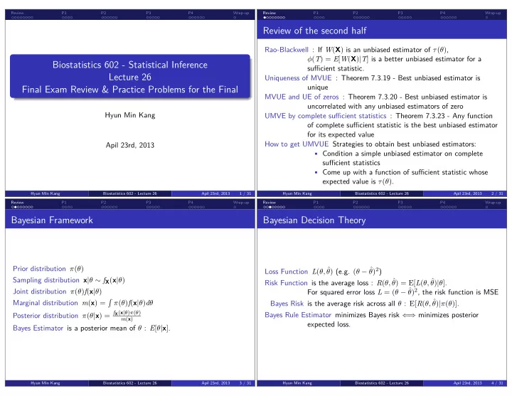
Bayesian Framework Biostatistics 602 - Lecture 26 of complete - PowerPoint PPT Presentation

. . . . . . . . P1 Wrap-up . P4 . . . . . . P3 . . . . . P2 . . . . . . . . . . Hyun Min Kang Review Review 2 / 31 Apil 23rd, 2013 Biostatistics 602 - Lecture 26 Hyun Min Kang sufficient statistics How to get UMVUE Strategies to obtain best unbiased estimators: Bayesian Framework Biostatistics 602 - Lecture 26 of complete sufficient statistic is the best unbiased estimator . . . . . . Apil 23rd, 2013 Biostatistics 602 - Lecture 26 Hyun Min Kang expected loss. Bayesian Decision Theory Wrap-up . P4 P3 Apil 23rd, 2013 . . . . . P2 . . . . . . P1 . . . . Review . . . . . . . . 3 / 31 for its expected value . . . . . . . . UMVE by complete sufficient statistics : Theorem 7.3.23 - Any function . Biostatistics 602 - Lecture 26 Hyun Min Kang Apil 23rd, 2013 Hyun Min Kang Final Exam Review & Practice Problems for the Final Lecture 26 Biostatistics 602 - Statistical Inference . Wrap-up uncorrelated with any unbiased estimators of zero . P4 . . . . . . P3 . . . . . P2 . . . . . . P1 . . . . Apil 23rd, 2013 1 / 31 . . . . . . . . P2 MVUE and UE of zeros : Theorem 7.3.20 - Best unbiased estimator is unique Uniqueness of MVUE : Theorem 7.3.19 - Best unbiased estimator is sufficient statistic. Review of the second half Wrap-up . P4 . . . . . . P3 . . . . . 4 / 31 . . . . . . P1 . . . . Review Rao-Blackwell : If W ( X ) is an unbiased estimator of τ ( θ ) , ϕ ( T ) = E [ W ( X ) | T ] is a better unbiased estimator for a • Condition a simple unbiased estimator on complete • Come up with a function of sufficient statistic whose expected value is τ ( θ ) . Prior distribution π ( θ ) Loss Function L ( θ, ˆ θ ) (e.g. ( θ − ˆ θ ) 2 ) Sampling distribution x | θ ∼ f X ( x | θ ) Risk Function is the average loss : R ( θ, ˆ θ ) = E [ L ( θ, ˆ θ ) | θ ] . For squared error loss L = ( θ − ˆ Joint distribution π ( θ ) f ( x | θ ) θ ) 2 , the risk function is MSE Bayes Risk is the average risk across all θ : E [ R ( θ, ˆ ∫ Marginal distribution m ( x ) = π ( θ ) f ( x | θ ) d θ θ ) | π ( θ )] . Posterior distribution π ( θ | x ) = f X ( x | θ ) π ( θ ) Bayes Rule Estimator minimizes Bayes risk ⇐ ⇒ minimizes posterior m ( x ) Bayes Estimator is a posterior mean of θ : E [ θ | x ] .

. . . . . . . . . . . . . test for one-sided composite hypothesis. Karlin-Rabin If T is sufficient and has MLR, then test rejecting Type II error given the upper bound of Type I error) UMP Wrap-up . P4 . . . . . . P3 P2 Biostatistics 602 - Lecture 26 . . . . . . P1 Review Review . . . . . . . . 6 / 31 Apil 23rd, 2013 Biostatistics 602 - Lecture 26 Hyun Min Kang Hyun Min Kang Apil 23rd, 2013 LRT based on sufficient statistics LRT based on full data and sufficient . Apil 23rd, 2013 Biostatistics 602 - Lecture 26 Hyun Min Kang p-value. valid p-value standard normal distribution d Asymptotic Tests and p-Values Wrap-up P4 7 / 31 . . . . . . P3 . . . . . P2 . . . . . . P1 . . . . Review . . . . . . . . statistics are identical. . . . . 8 / 31 Consistency Using law of large numbers, show variance and bias 5 / 31 Biostatistics 602 - Lecture 26 Hyun Min Kang asymptotically efficient under regularity condition. Asymptotic Efficiency of MLE Theorem 10.1.12 MLE is always Asymptotically Efficient ARE with CR-bound of unbiased estimator of V . Delta Method Asymptotic Normality Using central limit theorem, Slutsky Theorem, and Asymptotics Review Wrap-up . P4 . . . . . . P3 . . . . . P2 . . . . . . P1 . . . . . . . . . . . . Apil 23rd, 2013 . . . . P2 P1 Hypothesis Testing Wrap-up . P4 . . . . . . . . . . . . P3 . . . . . Type I error Pr ( X ∈ R | θ ) when θ ∈ Ω 0 Type II error 1 − Pr ( X ∈ R | θ ) when θ ∈ Ω c 0 converges to zero, for any continuous mapping function τ Power function β ( θ ) = Pr ( X ∈ R | θ ) β ( θ ) represents Type I error under H 0 , and power (=1-Type II error) under H 1 . Size α test sup θ ∈ Ω 0 β ( θ ) = α Asymptotic Relative Efficiency ARE ( V n , W n ) = σ 2 W / σ 2 Level α test sup θ ∈ Ω 0 β ( θ ) ≤ α LRT λ ( x ) = L (ˆ τ ( θ ) is 1. θ 0 | x ) rejects H 0 when λ ( x ) ≤ c L (ˆ θ | x ) ⇒ − 2 log λ ( x ) ≥ − 2 log c = c ∗ ⇐ Asymptotic Distribution of LRT For testing, H 0 : θ = θ 0 vs. H 1 : θ = θ 1 , Unbiased Test β ( θ 1 ) ≥ β ( θ 0 ) for every θ 1 ∈ Ω c 0 and θ 0 ∈ Ω 0 . → χ 2 − 2 log λ ( x ) 1 under regularity condition. UMP Test β ( θ ) ≥ β ′ ( θ ) for every θ ∈ Ω c 0 and β ′ ( θ ) of every other test Wald Test If W n is a consistent estimator of θ , and S 2 n is a consistent with a class of test C . estimator of Var ( W n ) , then Z n = ( W n − θ 0 )/ S n follows a UMP level α Test UMP test in the class of all the level α test. (smallest • Two-sided test : | Z n | > z α /2 • One-sided test : Z n > z α /2 or Z n < − z α /2 Neyman-Pearson For H 0 : θ = θ 0 vs. H 1 : θ = θ 1 , a test with rejection p-Value A p-value 0 ≤ p ( x ) ≤ 1 is valid if, Pr ( p ( X ) ≤ α | θ ) ≤ α for region f ( x | θ 1 )/ f ( x | θ 0 ) > k is a UMP level α test for its size. every θ ∈ Ω 0 and 0 ≤ α ≤ 1 . MLR g ( t | θ 2 )/ g ( t | θ 1 ) is an increasing function of t for every Constructing p-Value Theorem 8.3.27 : If large W ( X ) value gives evidence θ 2 > θ 1 . that H 1 is true, p ( x ) = sup θ ∈ Ω 0 Pr ( W ( X ) ≥ W ( x ) | θ ) is a R = { T : T > t 0 } or R = { T : T < t 0 } is an UMP level α p-Value given sufficient statistics For a sufficient statistic S ( X ) , p ( x ) = Pr ( W ( X ) ≥ W ( x ) | S ( X ) = S ( x )) is also a valid

. . . . . . . . P3 Hyun Min Kang Therefore, the family of X has an MLR. Review Solution for (a) Wrap-up . P4 . . . . . . . . . . . Apil 23rd, 2013 P2 . . . . . . P1 . . . . Review . . . . . . . . 10 / 31 Apil 23rd, 2013 Biostatistics 602 - Lecture 26 Biostatistics 602 - Lecture 26 11 / 31 (a) Show that this family has an MLR Wrap-up Apil 23rd, 2013 Biostatistics 602 - Lecture 26 Hyun Min Kang log e x X e Solution for (b) . . . . . . . . . P4 . . . . . . P3 . . . . . P2 . . . . . . P1 . . . . Review Hyun Min Kang 12 / 31 Biostatistics 602 - Lecture 26 Wrap-up P2 . . . . . . P3 . . . . . . P4 . Interval Estimation P3 P1 interval). Hyun Min Kang Apil 23rd, 2013 9 / 31 . . . . . . . . . . . . . . . . . . . . . . . P4 . . . . P1 . . . . . . P2 . . . . . Review . . Problem . Practice Problem 1 (continued from last week) Wrap-up . Let f ( x | θ ) be the logistic location pdf Coverage probability Pr ( θ ∈ [ L ( X ) , U ( X )]) e ( x − θ ) f ( x | θ ) − ∞ < x < ∞ , −∞ < θ < ∞ Coverage coefficient is 1 − α if inf θ ∈ Ω Pr ( θ ∈ [ L ( X ) , U ( X )]) = 1 − α = (1 + e ( x − θ ) ) 2 Confidence interval [ L ( X ) , U ( X )]) is 1 − α if inf θ ∈ Ω Pr ( θ ∈ [ L ( X ) , U ( X )]) = 1 − α Inverting a level α test If A ( θ 0 ) is the acceptance region of a level α test, (b) Based on one observation X , find the most powerful size α test of then C ( X ) = { θ : X ∈ A ( θ ) } is a 1 − α confidence set (or H 0 : θ = 0 versus H 1 : θ = 1 . (c) Show that the test in part (b) is UMP size α for testing H 0 : θ ≤ 0 vs. H 1 : θ > 0 . For θ 1 < θ 2 , The UMP test rejects H 0 if and only if ) 2 e ( x − θ 2) f ( x | 1) ( 1 + e x f ( x | θ 2 ) = (1+ e ( x − θ 2) ) 2 > k = f ( x | 0) 1 + e ( x − 1) f ( x | θ 1 ) e ( x − θ 1) 1 + e x (1+ e ( x − θ 1) ) 2 k ∗ > ) 2 1 + e ( x − 1) ( 1 + e ( x − θ 1 ) e ( θ 1 − θ 2 ) = 1 + e x k ∗∗ 1 + e ( x − θ 2 ) > e + e x > x 0 Let r ( x ) = (1 + e x − θ 1 )/(1 + e x − θ 2 ) Because under H 0 , F ( x 0 | θ = 0) = 1+ e x , the rejection region of UMP level e ( x − θ 1 ) (1 + e ( x − θ 2 ) ) − (1 + e ( x − θ 1 ) ) e ( x − θ 2 ) α test satisfies r ′ ( x ) = (1 + e ( x − θ 2 ) ) 2 1 1 − F ( x | θ = 0) = 1 + e x 0 = α e ( x − θ 1 ) − e ( x − θ 2 ) ( ∵ x − θ 1 > x − θ 2 ) = > 0 ( 1 − α ) (1 + e ( x − θ 2 ) ) 2 ∼ x 0 α