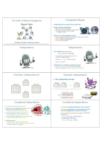
Bayes Net Representation CS 4100: Artificial Intelligence Bayes - PDF document

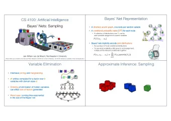
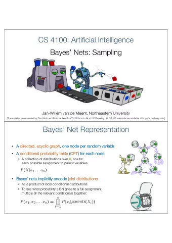
Bayes’ Net Representation CS 4100: Artificial Intelligence Bayes’ Nets: Sampling • A A di directed, d, acyclic graph ph, o , one n node p per r random v variable • A A co conditional al probab ability tab able (CP CPT) ) for each node de • A collection of distributions over X , one for each possible assignment to parent variables • Ba Bayes ’ ne nets implicitly enc ncode jo join int dis istrib ributio ions • As a product of local conditional distributions • To see what probability a BN gives to a full assignment, multiply all the relevant conditionals together: Jan-Willem van de Meent, Northeastern University [These slides were created by Dan Klein and Pieter Abbeel for CS188 Intro to AI at UC Berkeley. All CS188 materials are available at http://ai.berkeley.edu.] Variable Elimination Approximate Inference: Sampling • Interleave ve jo join inin ing and and marginalizi zing • d k entries s computed for a factor ove ver k va variables s with domain si size zes s d … • Or Orde dering of elimination of hidden va variables s … can af can affect ect si size ze of factors s ge generate ted • Worst st case se: running time exp xponential in the si in size ze of the Baye yes’ s’ net Sampling Sampling • Sampling is a lot like ke repeated simulation • Why Why sampl ple? • Example • Sampling from give u u = 0.83 ven dist stribution • Predicting the weather, basketball games, … • Re Reinforcement Learning: Can C P(C) • St Step p 1: Get sample u from uniform approximate (q-)values even when distribution over [0 [0, 1) 0 0.6 0.7 1.0 red 0.6 you don’t know the transition function • Ba Basic idea • E.g. ra random() m() in python • In Inference: : getting a sample is faster than green 0.1 • Dr Draw N samples from a sampling distribution S • St Step p 2: Convert this sample u into computing the right answer (e.g. with blue 0.3 an outcome for the given distribution • Co Compute an approximate posterior probability variable elimination) by having each target outcome • Show this co conver verges ges to the true probability P associated with a sub-interval of [0 [0,1) with sub-interval size equal to • If ra random() returns u = = 0.83 , probability of the outcome then our sample is C = = blue • E.g, after sampling 8 times: Sampling in Bayes’ Nets Prior Sampling • Pr Prior ior Sa Samp mplin ling • Re Rejecti tion Sampling • Like kelihood Weighting • Gi Gibbs Sampling

Prior Sampling Prior Sampling +c 0.5 • For For i = 1 , 2 , …, n -c 0.5 • Sa Sampl ple x i fr from P( P(X i | Parents( s(X i )) )) Cloudy Cloudy +c +s 0.1 +c +r 0.8 • Re Return (x (x 1 , x , x 2 , …, …, x n ) -s 0.9 -r 0.2 +s 0.5 +r 0.2 -c -c Sprinkler Sprinkler Rain Rain -s 0.5 -r 0.8 Samples: WetGrass WetGrass +w 0.99 +s +r -w 0.01 +c, -s, +r, +w -r +w 0.90 -c, +s, -r, +w -w 0.10 … +r +w 0.90 -s -w 0.10 -r +w 0.01 -w 0.99 Example Prior Sampling • This s process ss generates s sa samples s with pr proba babi bility ty: • We We’ll ll dr draw w a ba batch of sa samples f s from t the B BN: +c, -s, +r +c +r, +w +w C +c, +s +c +s, +r +r, +w +w S R -c, +s +s, +r +r, -w … i.e … .e. th . the B BN’s s joint probability +c, -s, +r +c +r, +w +w W -c, c, -s, s, -r, +w +w • Let the number of sa samples s of an eve vent be • If we want to kn know P( P(W) • Co Count outcomes <+ <+w: 4 : 4, , -w: 1 : 1> • Then Then • No Normaliz lize to get P(W) = = <+w <+w: 0 : 0.8 .8, , -w: 0 : 0.2 .2> • Estimate will get closer to the true distribution with more samples • Can estimate anything else, too • What about P(C | +w +w) ? P( P(C | +r, r, +w +w) ? P( P(C | -r, r, -w) ? • i.e., the sa sampling procedure is s consi sist stent* • Fa Fast st: can use fewer samples if less time (what’s the drawback?) (different from consi sist stent heurist stic, or arc consi sist stency) y) Rejection Sampling Rejection Sampling • Le Let’ t’s s sa say y we want P( P(C) • No point keeping all samples around C • Just tally counts of C as we go S R W • Le Let’ t’s s sa say y we want P( P(C | +s) • Sa Same me id idea: tally C outcomes, but ignore +c +c, -s, +r +r, +w +w (reject) samples which don’t have S= S=+s +c +c, +s +s, +r +r, +w +w • This is called re reje jectio ion samplin ling -c, +s +s, +r +r, -w +c, -s, +r +c +r, +w +w • It is also consistent for conditional probabilities -c, c, -s, s, -r, +w +w (i.e., correct in the limit of large N ) Rejection Sampling Likelihood Weighting • In Input: t: evidence assignments • For For i = 1, 2, …, …, n • Sa Sample mple x i fr from om P(X P(X i | Parents( s(X i )) )) • If x i not consi If sist stent with evi vidence • Re Reje ject: Return – no sample is generated in this cycle • Re Return (x (x 1 , x , x 2 , …, …, x n )