Basic Framework [Most of this lecture from Sutton & Barto] The - PowerPoint PPT Presentation

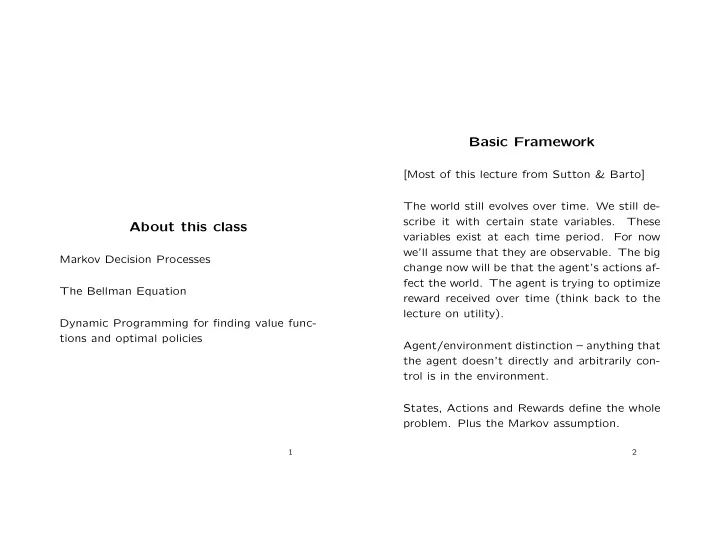
Basic Framework [Most of this lecture from Sutton & Barto] The world still evolves over time. We still de- scribe it with certain state variables. These About this class variables exist at each time period. For now we’ll assume that they are observable. The big Markov Decision Processes change now will be that the agent’s actions af- fect the world. The agent is trying to optimize The Bellman Equation reward received over time (think back to the lecture on utility). Dynamic Programming for finding value func- tions and optimal policies Agent/environment distinction – anything that the agent doesn’t directly and arbitrarily con- trol is in the environment. States, Actions and Rewards define the whole problem. Plus the Markov assumption. 1 2

We’ll usually see two di ff erent types of reward MDPs: Mathematical Structure structures – big reward at the end, or “flow” rewards as time goes on. What do we need to know? We’re going to deal with two di ff erent kinds of Transition probabilities (now dependent on ac- problems: episodic and continuing. tions!) P a ss ′ = Pr( s t +1 = s ′ | s t = s, a t = a ) The reward the agent tries to optimize for an episodic task can just be the sum of individual rewards over time. Expected rewards R a ss ′ = E [ r t +1 | s t = s, a t = a, s t +1 = s ′ ] The reward the agent tries to optimize for a continuing task must be discounted. Rewards are sometimes associated with states and sometimes with (State, Action) pairs. The MDP and it’s partially observable cousin the POMDP, are the standard representation Note: we lose distribution information about for many problems in control, economics, robotics, rewards in this formulation. etc. 3

Policies and Value Functions A policy is a mapping from (State, Action) pairs to probabilities. π ( s, a ) = prob. of taking action a in state s ∞ γ k r t + k +2 | s t = s ] � V π ( s ) = E π [ r t +1 + γ States have values under policies. k =0 V π ( s ) = E π [ R t | s t = s ] ∞ P a ss ′ [ R a γ k r t + k +2 | s t = s ]] � � � = π ( s, a ) ss ′ + γ E π [ ∞ γ k r t + k +1 | s t = s ] � = E π [ a s ′ k =0 k =0 P a ss ′ [ R a ss ′ + γ V π ( s ′ )] � � = π ( s, a ) a s ′ It is also sometimes useful to define an action- value function: This is the Bellman equation for V π Q π ( s, a ) = E π [ R t | s t = s, a t = a ] Note that in this definition we fix the current action, and then follow policy π Finding the value function for a policy: 4

An Example: Gridworld Actions: L,R,U,D If you try to move o ff the grid you don’t go anywhere. The top left and bottom right corners are ab- sorbing states. 0 -14 -20 -22 -14 -18 -20 -20 The task is episodic and undiscounted. Each -20 -20 -18 -14 transition earns a reward of -1, except that -22 -20 -14 0 you’re finished when you enter an absorbing state A A What is the value function of the policy π that takes each action equiprobably in each state? 5

Optimal Policies One policy is better than another if it’s ex- Dynamic Programming pected return is greater across all states. An optimal policy is one that is better than or equal to all other policies. How do we solve for the optimal value func- tion? We turn the Bellman equations into up- date rules that converge. V ∗ ( s ) = max V π ( s ) π Keep in mind: we must know model dynamics Bellman optimality equation: the value of a perfectly for these methods to be correct. state under an optimal policy must equal the expected return of taking the best action from that state. Two key cogs: V ∗ ( s ) = max E [ r t +1 + γ V ∗ ( s ′ ) | a t = a ] a 1. Policy evaluation P a ss ′ ( R a ss ′ + γ V ∗ ( s ′ )) � = max a s ′ 2. Policy improvement Given the optimal value function, it is easy to compute the actions that implement the opti- mal policy. V ∗ allows you to solve the problem greedily! 6 7

Policy Evaluation i. v ← V ( s ) How do we derive the value function for any s ′ P a ss ′ [ R a ss ′ + γ V ( s ′ )] ii. V ( s ) ← � a π ( s, a ) � policy, leave alone an optimal one? If you think about it, Actually works faster when you update the ar- ray in place instead of maintaining two sepa- P a ss ′ [ R a ss ′ + γ V π ( s ′ )] � � V π ( s ) = π ( s, a ) rate arrays for the sweep over the state space! a s ′ is a system of linear equations. Back to Gridworld and the equiprobable action selection policy: We use an iterative solution method. The Bell- man equation tells us there is a solution, and it 0 0 0 0 turns out that solution will be the fixed point of 0 0 0 0 an iterative method that operates as follows: t = 0 : 0 0 0 0 0 0 0 0 1. Initialize V ( s ) ← 0 for all s 0 -1 -1 -1 -1 -1 -1 -1 t = 1 : 2. Repeat until convergence -1 -1 -1 -1 -1 -1 -1 0 (a) For all states s 8

Policy Improvement 0 -1.7 -2.0 -2.0 Suppose you have a deterministic policy π and -1.7 -2.0 -2.0 -2.0 t = 2 : -2.0 -2.0 -2.0 -1.7 want to improve on it. How about choosing a -2.0 -2.0 -1.7 0 in state s and then continuing to follow π ? 0 -2.4 -2.9 -3.0 Policy improvement theorem: -2.4 -2.9 -3.0 -2.9 t = 3 : -2.9 -3.0 -2.9 -2.4 If Q π ( s, π ′ ( s )) ≥ V π ( s ) for all states s , then: -3.0 -2.9 -2.4 0 V π ′ ( s ) ≥ V π ( s ) 0 -6.1 -8.4 -9.0 -6.1 -7.7 -8.4 -8.4 t = 10 : Relatively easy to prove by repeated expansion -8.4 -8.4 -7.7 -6.1 of Q π ( s, π ′ ( s )). -9.0 -8.4 -6.1 0 Consider a short-sighted greedy improvement 0 -14 -20 -22 to the policy π , in which, at each state we -14 -18 -20 -20 t = ∞ : -20 -20 -18 -14 choose the action that appears best according -22 -20 -14 0 to Q π ( s, a ) π ′ ( s, a ) = arg max Q π ( s, a ) a 9

P a ss ′ [ R a ss ′ + γ V π ( s ′ )] � = arg max a s ′ What would policy improvement in the Grid- world example yield? L L L/D U L/U L/D D This is the Bellman optimality equation, and therefore V π ′ must be V ∗ . U U/R R/D D U/R R R The policy improvement theorem generalizes Note that this is the same thing that would to stochastic policies under the definition: happen from t = 3 onwards! Q π ( s, π ′ ( s )) = π ′ ( s, a ) Q π ( s, a ) � Only guaranteed to be an improvement over a the random policy but in this case it happens to also be optimal. If the new policy π ′ is no better than π then it must be true for all s that V π ′ ( s ) = max ss ′ + γ V π ′ ( s ′ )] P a ss ′ [ R a � a s ′

Policy Iteration Interleave the steps. Start with a policy, eval- uate it, then improve it, then evaluate the new policy, improve it, etc., until it stops changing. 3. Perform policy improvement: E → V π 0 I E → · · · I → π ∗ E → V ∗ P π ( s ) [ R π ( s ) + γ V ( s ′ )] − − → π 1 − − − � π ( s ) ← arg max π 0 ss ′ ss ′ a s ′ If the policy is the same as last time then Algorithm: you are done! 1. Initialize with arbitrary value function and Takes very few iterations in practice, even though policy the policy evaluation step is itself iterative. 2. Perform policy evaluation to find V π ( s ) for all s ∈ S . That is, repeat the following update until convergence P π ( s ) [ R π ( s ) + γ V ( s ′ )] � V ( s ) ← ss ′ ss ′ s ′ 10

Value Iteration Discussion of Dynamic Initialize V arbitrarily Programming Repeat until convergence: We can solve MDPs with millions of states. Ef- ficiency isn’t as bad as you’ll sometimes hear. For each s ∈ S There is a problem in that the state repre- sentation must be relatively compact. If your s ′ P a ss ′ [ R a ss ′ + γ V ( s ′ )] • V ( s ) ← max a � state representation, and hence your number of states, grows very fast, then you’re in trou- Output policy π such that ble. But that’s a feature of the problem, not P a ss ′ [ R a ss ′ + γ V ( s ′ )] the method. � π ( s ) = arg max a s ′ Asynchronous dynamic programming: a lead Convergence criterion: the maximum change in... in the value of any state in the state set in the last iteration was less than some threshold Instead of doing sweeps of the whole state space at each iteration, just use whatever val- Note that this is simply turning the Bellman equation into an update rule! It can also be ues are available at any time to update any thought of as an update that cuts o ff policy state. In place algorithms. evaluation after one step... 11 12

Convergence has to be handled carefully, be- cause in general convergence to the value func- tion only occurs if we then visit all states in- finitely often in the limit – so we can’t stop going to certain states if we want the guaran- tee to hold. But we can run an iterative DP algorithm on- line at the same time that the agent is actually in the MDP. Could focus on important regions of the state space, perhaps at the expense of true convergence? What’s next? What if we don’t have a correct model of the MDP? How do we build one while also acting? We’ll start by going through really simple MDPs, namely Bandit problems.