Basic Framework [This lecture adapted from Sutton & Barto and - PDF document

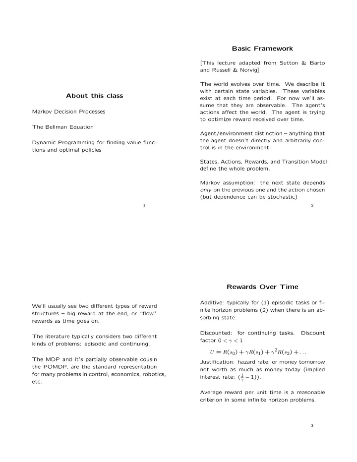
Basic Framework [This lecture adapted from Sutton & Barto and Russell & Norvig] The world evolves over time. We describe it with certain state variables. These variables About this class exist at each time period. For now we’ll as- sume that they are observable. The agent’s Markov Decision Processes actions a ff ect the world. The agent is trying to optimize reward received over time. The Bellman Equation Agent/environment distinction – anything that the agent doesn’t directly and arbitrarily con- Dynamic Programming for finding value func- trol is in the environment. tions and optimal policies States, Actions, Rewards, and Transition Model define the whole problem. Markov assumption: the next state depends only on the previous one and the action chosen (but dependence can be stochastic) 1 2 Rewards Over Time Additive: typically for (1) episodic tasks or fi- We’ll usually see two di ff erent types of reward nite horizon problems (2) when there is an ab- structures – big reward at the end, or “flow” sorbing state. rewards as time goes on. Discounted: for continuing tasks. Discount The literature typically considers two di ff erent factor 0 < γ < 1 kinds of problems: episodic and continuing. U = R ( s 0 ) + γ R ( s 1 ) + γ 2 R ( s 2 ) + . . . The MDP and it’s partially observable cousin Justification: hazard rate, or money tomorrow the POMDP, are the standard representation not worth as much as money today (implied for many problems in control, economics, robotics, interest rate: ( 1 γ � 1)). etc. Average reward per unit time is a reasonable criterion in some infinite horizon problems. 3

MDPs: Mathematical Structure What do we need to know? Transition probabilities (now dependent on ac- Policies tions!) A fixed set of actions won’t solve the problem P a ss 0 = Pr( s t +1 = s 0 | s t = s, a t = a ) (why? nondeterministic!) Expected rewards A policy is a mapping from (State, Action) R a ss 0 = E [ r t +1 | s t = s, a t = a, s t +1 = s 0 ] pairs to probabilities. π ( s, a ) = prob. of taking action a in state s . Rewards are sometimes associated with states and sometimes with (State, Action) pairs. Note: we lose distribution information about rewards in this formulation. 4 5 Example: Motion Planning +1 -1 We have two absorbing states and one square R ( s ) = � 0 . 04 you can’t get to. ! ! ! +1 Actions: N, E, W, S. -1 " " " Transition model: With Pr(0 . 8) you go in the direction you intend (an action that would move What about R ( s ) = � 0 . 001? into walls or the gray square instead leaves you where you were). With Pr(0 . 1) you instead go in each perpendicular direction. Optimal policy? Depends on the per-time-step reward! 6 7

R ( s ) = � 0 . 001 R ( s ) = � 1 . 7 ! ! ! +1 ! ! ! +1 -1 -1 " " ! " # ! ! ! " What about R ( s ) = � 1 . 7? What about R ( s ) > 0? 8 9 Policies and Value Functions Remember π ( s, a ) = prob. of taking action a in state s States have values under policies. 1 V π ( s ) = E π [ R t | s t = s ] V π ( s ) = E π [ r t +1 + γ γ k r t + k +2 | s t = s ] X k =0 1 γ k r t + k +1 | s t = s ] X = E π [ 1 P a ss 0 [ R a γ k r t + k +2 | s t = s ]] k =0 X X X = π ( s, a ) ss 0 + γ E π [ a s 0 k =0 It is also sometimes useful to define an action- P a ss 0 [ R a ss 0 + γ V π ( s 0 )] X X = π ( s, a ) value function: a s 0 Q π ( s, a ) = E π [ R t | s t = s, a t = a ] Note that in this definition we fix the current action, and then follow policy π Finding the value function for a policy: 10

Optimal Policies One policy is better than another if it’s ex- pected return is greater across all states. An optimal policy is one that is better than or equal to all other policies. Given the optimal value function, it is easy to V ⇤ ( s ) = max V π ( s ) π compute the actions that implement the opti- mal policy. V ⇤ allows you to solve the problem Bellman optimality equation: the value of a greedily! state under an optimal policy must equal the expected return of taking the best action from that state, and then following the optimal pol- icy. V ⇤ ( s ) = max E [ r t +1 + γ V ⇤ ( s 0 ) | a t = a ] a P a ss 0 ( R a ss 0 + γ V ⇤ ( s 0 )) X = max a s 0 11 Policy Evaluation How do we derive the value function for any Dynamic Programming policy, leave alone an optimal one? How do we solve for the optimal value func- If you think about it, tion? We turn the Bellman equations into up- V π ( s ) = P a ss 0 [ R a ss 0 + γ V π ( s 0 )] X X π ( s, a ) date rules that converge. a s 0 is a system of linear equations. Keep in mind: we must know model dynamics perfectly for these methods to be correct. We use an iterative solution method. The Bell- man equation tells us there is a solution, and it Two key cogs: turns out that solution will be the fixed point of an iterative method that operates as follows: 1. Policy evaluation 1. Initialize V ( s ) 0 for all s 2. Policy improvement 2. Repeat until convergence ( | v � V ( S ) | < δ ) (a) For all states s 12 13

An Example: Gridworld Actions: L,R,U,D If you try to move o ff the grid you don’t go anywhere. i. v V ( s ) The top left and bottom right corners are ab- sorbing states. s 0 P a ss 0 [ R a ss 0 + γ V ( s 0 )] ii. V ( s ) P a π ( s, a ) P The task is episodic and undiscounted. Each transition earns a reward of -1, except that Actually works faster when you update the ar- you’re finished when you enter an absorbing ray in place instead of maintaining two sepa- state rate arrays for the sweep over the state space! A A What is the value function of the policy π that takes each action equiprobably in each state? 14 0 0 0 0 0 0 0 0 t = 0 : 0 0 0 0 0 0 0 0 0 -1 -1 -1 -1 -1 -1 -1 t = 1 : -1 -1 -1 -1 -1 -1 -1 0 0 -1.7 -2.0 -2.0 0 -14 -20 -22 -1.7 -2.0 -2.0 -2.0 -14 -18 -20 -20 t = 2 : t = 1 : -2.0 -2.0 -2.0 -1.7 -20 -20 -18 -14 -2.0 -2.0 -1.7 0 -22 -20 -14 0 0 -2.4 -2.9 -3.0 -2.4 -2.9 -3.0 -2.9 t = 3 : -2.9 -3.0 -2.9 -2.4 -3.0 -2.9 -2.4 0 0 -6.1 -8.4 -9.0 -6.1 -7.7 -8.4 -8.4 t = 10 : -8.4 -8.4 -7.7 -6.1 -9.0 -8.4 -6.1 0

P a ss 0 [ R a ss 0 + γ V π ( s 0 )] Policy Improvement = arg max X a s 0 Suppose you have a deterministic policy π and What would policy improvement in the Grid- want to improve on it. How about choosing a world example yield? in state s and then continuing to follow π ? L L L/D Policy improvement theorem: U L/U L/D D U U/R R/D D If Q π ( s, π 0 ( s )) � V π ( s ) for all states s , then: U/R R R V π 0 ( s ) � V π ( s ) Note that this is the same thing that would happen from t = 3 onwards! Relatively easy to prove by repeated expansion of Q π ( s, π 0 ( s )). Only guaranteed to be an improvement over the random policy but in this case it happens to also be optimal. Consider a short-sighted greedy improvement to the policy π , in which, at each state we If the new policy π 0 is no better than π then it choose the action that appears best according must be true for all s that to Q π ( s, a ) V π 0 ( s ) = max ss 0 + γ V π 0 ( s 0 )] P a ss 0 [ R a X π 0 ( s, a ) = arg max Q π ( s, a ) a s 0 a 15 Policy Iteration Interleave the steps. Start with a policy, eval- uate it, then improve it, then evaluate the new policy, improve it, etc., until it stops changing. This is the Bellman optimality equation, and E ! V π 0 I E ! · · · I ! π ⇤ E therefore V π 0 must be V ⇤ . ! V ⇤ π 0 � � ! π 1 � � � Algorithm: The policy improvement theorem generalizes to stochastic policies under the definition: Q π ( s, π 0 ( s )) = π 0 ( s, a ) Q π ( s, a ) X 1. Initialize with arbitrary value function and a policy 2. Perform policy evaluation to find V π ( s ) for all s 2 S . That is, repeat the following update until convergence P π ( s ) [ R π ( s ) + γ V ( s 0 )] X V ( s ) ss 0 ss 0 s 0 16