Baseline accuracy: 74.4% Top 3 features: Top 3 students: Male sex - PowerPoint PPT Presentation

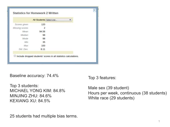
Baseline accuracy: 74.4% Top 3 features: Top 3 students: Male sex (39 student) MICHAEL YONG KIM: 84.8% Hours per week, continuous (38 students) MINJING ZHU: 84.6% White race (29 students) KEXIANG XU: 84.5% ​ 25 students had multiple bias terms ​ . 1

CSE446: ¡Ensemble ¡Learning ¡-­‑ ¡ Bagging ¡and ¡Boos7ng ¡ Winter ¡2016 ¡ Ali ¡Farhadi ¡ ¡ ¡ Slides ¡adapted ¡from ¡Carlos ¡Guestrin, ¡Nick ¡Kushmerick, ¡Padraig ¡ Cunningham, ¡and ¡Luke ¡ZeKlemoyer ¡ ¡

3

4

Vo7ng ¡ ¡(Ensemble ¡Methods) ¡ • Instead ¡of ¡learning ¡a ¡single ¡classifier, ¡learn ¡ many ¡ weak ¡classifiers ¡that ¡are ¡ good ¡at ¡different ¡parts ¡of ¡ the ¡data ¡ • Output ¡class: ¡ (Weighted) ¡vote ¡of ¡each ¡classifier ¡ – Classifiers ¡that ¡are ¡most ¡“sure” ¡will ¡vote ¡with ¡more ¡ convic7on ¡ – Classifiers ¡will ¡be ¡most ¡“sure” ¡about ¡a ¡par7cular ¡part ¡of ¡ the ¡space ¡ – On ¡average, ¡do ¡beKer ¡than ¡single ¡classifier! ¡ • But ¡how??? ¡ ¡ – force ¡classifiers ¡to ¡learn ¡about ¡different ¡parts ¡of ¡the ¡input ¡ space? ¡different ¡subsets ¡of ¡the ¡data? ¡ – weigh ¡the ¡votes ¡of ¡different ¡classifiers? ¡

BAGGing = Bootstrap AGGregation (Breiman, 1996) • for i = 1, 2, …, K: – T i � randomly select M training instances with replacement – h i � learn(T i ) [Decision Tree, Naive Bayes, …] • Now combine the h i together with uniform voting (w i =1/K for all i)

7

decision tree learning algorithm; very similar to version in earlier slides 8

shades of blue/red indicate strength of vote for particular classification

Figh7ng ¡the ¡bias-­‑variance ¡tradeoff ¡ • Simple ¡(a.k.a. ¡weak) ¡learners ¡are ¡good ¡ – e.g., ¡naïve ¡Bayes, ¡logis7c ¡regression, ¡decision ¡ stumps ¡(or ¡shallow ¡decision ¡trees) ¡ – Low ¡variance, ¡don’t ¡usually ¡overfit ¡ • Simple ¡(a.k.a. ¡weak) ¡learners ¡are ¡bad ¡ – High ¡bias, ¡can’t ¡solve ¡hard ¡learning ¡problems ¡ • Can ¡we ¡make ¡weak ¡learners ¡always ¡good??? ¡ – No!!! ¡ – But ¡oCen ¡yes… ¡

Boos7ng ¡ [Schapire, 1989] • Idea: ¡given ¡a ¡weak ¡learner, ¡run ¡it ¡mul7ple ¡7mes ¡on ¡ (reweighted) ¡training ¡data, ¡then ¡let ¡learned ¡classifiers ¡vote ¡ • On ¡each ¡itera7on ¡ t : ¡ ¡ – weight ¡each ¡training ¡example ¡by ¡how ¡incorrectly ¡it ¡was ¡ classified ¡ – Learn ¡a ¡hypothesis ¡– ¡h t ¡ – A ¡strength ¡for ¡this ¡hypothesis ¡– ¡ α t ¡ ¡ � ⇥ • Final ¡classifier: ¡ h ( x ) = sign α i h i ( x ) i • PracFcally ¡useful ¡ • TheoreFcally ¡interesFng ¡

time = 0 blue/red = class size of dot = weight weak learner = Decision stub: horizontal or vertical l 13

time = 1 this hypothesis has 15% error and so does this ensemble, since the ensemble contains just this one hypothesis 14

time = 2 15

time = 3 16

time = 13 17

time = 100 18

time = 300 overfitting!! 19

Learning ¡from ¡weighted ¡data ¡ • Consider ¡a ¡weighted ¡dataset ¡ – D(i) ¡– ¡weight ¡of ¡ i ¡ th ¡training ¡example ¡( x i ,y i ) ¡ – Interpreta7ons: ¡ • i ¡ th ¡training ¡example ¡counts ¡as ¡if ¡it ¡occurred ¡D(i) ¡7mes ¡ • If ¡I ¡were ¡to ¡“resample” ¡data, ¡I ¡would ¡get ¡more ¡samples ¡of ¡ “heavier” ¡data ¡points ¡ • Now, ¡always ¡do ¡weighted ¡calculaFons: ¡ – e.g., ¡MLE ¡for ¡Naïve ¡Bayes, ¡redefine ¡ Count(Y=y) ¡to ¡be ¡weighted ¡count: ¡ n D ( j ) δ ( Y j = y ) Count ( Y = y ) = j =1 – sebng ¡D(j)=1 ¡(or ¡any ¡constant ¡value!), ¡for ¡all ¡j, ¡will ¡recreates ¡ unweighted ¡case ¡

Given: ¡ ( x 1 , y 1 ) , . . . , ( x m , y m ) where x i ∈ R n , y i ∈ { − 1 , +1 } Ini7alize: ¡ D 1 ( i ) = 1 /m, for i = 1 , . . . , m How? Many possibilities. Will For ¡t=1…T: ¡ see one shortly! • Train ¡base ¡classifier ¡h t (x) ¡using ¡D t ¡ Why? Reweight the data: examples i that are • Choose ¡α t ¡ misclassified will have • Update, ¡for ¡i=1..m: ¡ higher weights! D t +1 ( i ) ∝ D t ( i ) exp( − α t y i h t ( x i )) with ¡normaliza7on ¡constant: ¡ • y i h t (x i ) > 0 � h i correct m ¡ • y i h t (x i ) < 0 � h i wrong X D t ( i ) exp( − α t y i h t ( x i )) • h i correct, α t > 0 � ¡ i =1 D t+1 (i) < D t (i) ¡ Output ¡final ¡classifier: ¡ • h i wrong, α t > 0 � T ! D t+1 (i) > D t (i) X H ( x ) = sign α t h t ( x ) i =1 Final Result: linear sum of “base” or “weak” classifier outputs.

m Given: ¡ ( x 1 , y 1 ) , . . . , ( x m , y m ) where x i ∈ R n , y i ∈ { − 1 , +1 } X D t ( i ) � ( h t ( x i ) 6 = y i ) ✏ t = Ini7alize: ¡ D 1 ( i ) = 1 /m, for i = 1 , . . . , m i =1 For ¡t=1…T: ¡ • Train ¡base ¡classifier ¡h t (x) ¡using ¡D t ¡ • Choose ¡α t ¡ • Update, ¡for ¡i=1..m: ¡ D t +1 ( i ) ∝ D t ( i ) exp( − α t y i h t ( x i )) ¡ • ε t : ¡error ¡of ¡h t , ¡weighted ¡by ¡D t ¡ ¡ • 0 ≤ ε t ≤ 1 ¡ 2 • α t : 1 α t • No ¡errors: ε t =0 ¡ � ¡ α t = ∞ 0.2 0.4 0.6 0.8 1.0 � 1 • All ¡errors: ¡ ε t = 1 ¡ � ¡ α t = −∞ � 2 • Random: ¡ ε t = 0.5 ¡ � α t =0 ¡ ε t � 3 m) on

What ¡ α t ¡to ¡choose ¡for ¡hypothesis ¡ h t ? ¡ [Schapire, 1989] Idea: ¡choose ¡ α t ¡to ¡minimize ¡a ¡bound ¡on ¡training ¡error! ¡ ¡ m m X X δ ( H ( x i ) 6 = y i )  D t ( i ) exp( � y i f ( x i )) ¡ ¡ i =1 i =1 Where ¡ ¡ ¡ ¡ ¡ exp( − y i f ( x i )) δ ( H ( x i ) 6 = y i ) y i f ( x i )

What ¡ α t ¡to ¡choose ¡for ¡hypothesis ¡ h t ? ¡ [Schapire, 1989] Idea: ¡choose ¡ α t ¡to ¡minimize ¡a ¡bound ¡on ¡training ¡error! ¡ ¡ m m 1 δ ( H ( x i ) 6 = y i )  1 Y X X D t ( i ) exp( � y i f ( x i )) Z t ¡ = m m ¡ i =1 i =1 t Where ¡ ¡ ¡ This equality isn’t And ¡ ¡ m obvious! Can be ¡ X D t ( i ) exp( − α t y i h t ( x i )) Z t = shown with algebra ¡ (telescoping sums)! i =1 ¡ If ¡we ¡minimize ¡ ∏ t ¡Z t , ¡we ¡minimize ¡our ¡training ¡error!!! ¡ • We ¡can ¡7ghten ¡this ¡bound ¡greedily, ¡by ¡choosing ¡ α t ¡and ¡ h t ¡ on ¡each ¡itera7on ¡to ¡minimize ¡ Z t . • h t ¡is ¡es7mated ¡as ¡a ¡black ¡box, ¡but ¡can ¡we ¡solve ¡for ¡ α t ?

Summary: ¡choose ¡ α t ¡ to ¡minimize ¡ error ¡bound ¡ ¡ [Schapire, 1989] We ¡can ¡squeeze ¡this ¡bound ¡by ¡choosing ¡ α t ¡on ¡each ¡ itera7on ¡to ¡minimize ¡ Z t . m ¡ X D t ( i ) exp( − α t y i h t ( x i )) Z t = ¡ m i =1 X D t ( i ) � ( h t ( x i ) 6 = y i ) ✏ t = ¡ i =1 For ¡boolean ¡Y: ¡differen7ate, ¡set ¡equal ¡to ¡0, ¡there ¡is ¡a ¡ closed ¡form ¡solu7on! ¡[Freund ¡& ¡Schapire ¡’97]: ¡ ¡ ¡ ¡ ¡ ¡ ¡ ¡

Ini7alize: ¡ D 1 ( i ) = 1 /m, for i = 1 , . . . , m Use ¡decision ¡stubs ¡as ¡base ¡classifier ¡ For ¡t=1…T: ¡ Ini7al: ¡ Train ¡base ¡classifier ¡h t (x) ¡using ¡D t ¡ • D 1 ¡= ¡[D 1 (1), ¡D 1 (2), ¡D 1 (3)] ¡= ¡[.33,.33,.33] ¡ • t=1: ¡ Choose ¡α t ¡ • m X D t ( i ) � ( h t ( x i ) 6 = y i ) ✏ t = Train ¡stub ¡[work ¡omiKed, ¡breaking ¡7es ¡randomly] ¡ • h 1 (x)=+1 ¡if ¡x 1 >0.5, ¡-­‑1 ¡otherwise ¡ • i =1 ¡ ¡ ε 1 =Σ i D 1 (i) ¡δ(h 1 (x i )≠y i ) ¡ ¡ • ¡= ¡0.33×1+0.33×0+0.33×0=0.33 ¡ Update, ¡for ¡i=1..m: ¡ • α 1 =(1/2) ¡ln((1-­‑ε 1 )/ε 1 )=0.5×ln(2)= ¡0.35 ¡ • ¡ D t +1 ( i ) ∝ D t ( i ) exp( − α t y i h t ( x i )) D 2 (1) ¡α ¡D 1 (1)×exp(-­‑α 1 y 1 h 1 (x 1 )) ¡ • Output ¡final ¡classifier : ¡ = ¡0.33×exp(-­‑0.35×1×-­‑1) ¡= ¡0.33 × exp(0.35) ¡= ¡0.46 ¡ D 2 (2) ¡α ¡D 1 (2) ¡× ¡exp(-­‑α 1 y 2 h 1 (x 2 )) ¡ ¡ T ! • X H ( x ) = sign α t h t ( x ) = ¡0.33×exp(-­‑0.35×-­‑1×-­‑1) ¡= ¡0.33 × exp(-­‑0.35) ¡= ¡0.23 ¡ i =1 D 2 (3) ¡α ¡D 1 (3) ¡× ¡exp(-­‑α 1 y 3 h 1 (x 3 )) ¡ • x 1 ¡ y ¡ = ¡0.33×exp(-­‑0.35×1×1) ¡= ¡0.33 × exp(-­‑0.35) ¡=0.23 ¡ D 2 ¡ = ¡[D 1 (1), ¡D 1 (2), ¡D 1 (3)] ¡= ¡[0.5,0.25,0.25] ¡ • -­‑1 ¡ 1 ¡ t=2 ¡ Con7nues ¡on ¡next ¡slide! ¡ • x 1 0 ¡ -­‑1 ¡ 1 ¡ 1 ¡ H(x) = sign(0.35 × h 1 (x)) ¡ • h 1 (x)=+1 if x 1 >0.5, -1 otherwise ¡