Bandit Optimisation with Approximations Kirthevasan Kandasamy - PowerPoint PPT Presentation

Multi-fidelity Bandit Optimisation in 2 Fidelities (1 Approximation) (Kandasamy et al. NIPS 2016b) f (2) f (1) x ⋆ At time t : Determine the point x t ∈ X and fidelity m t ∈ { 1 , 2 } for querying. Maximise f (2) . Don’t care for maximum of f (1) . End Goal: S (Λ) = f (2) ( x ⋆ ) − max t : m t =2 f (2) ( x t ) Simple Regret: S (Λ) = + ∞ if we haven’t queried f (2) yet. → But use f (1) to guide search for x ⋆ at f (2) . 11/26

Challenges f (2) = f x ⋆ 11/26

Challenges f (2) + ζ (1) − ζ (1) x ⋆ 11/26

Challenges f (2) f (1) x ⋆ 11/26

Challenges f (2) f (1) x ⋆ ◮ f (1) is not just a noisy version of f (2) . 11/26

Challenges f (2) f (1) x ⋆ x (1) ⋆ ◮ f (1) is not just a noisy version of f (2) . x (1) ◮ Cannot just maximise f (1) . is suboptimal for f (2) . ⋆ 11/26

Challenges f (2) f (1) x ⋆ x (1) ⋆ ◮ f (1) is not just a noisy version of f (2) . x (1) ◮ Cannot just maximise f (1) . is suboptimal for f (2) . ⋆ 11/26

Challenges f (2) f (1) x ⋆ x (1) ⋆ ◮ f (1) is not just a noisy version of f (2) . x (1) ◮ Cannot just maximise f (1) . is suboptimal for f (2) . ⋆ 11/26

Challenges f (2) f (1) x ⋆ x (1) ⋆ ◮ f (1) is not just a noisy version of f (2) . x (1) ◮ Cannot just maximise f (1) . is suboptimal for f (2) . ⋆ 11/26

Challenges f (2) f (1) x ⋆ x (1) ⋆ ◮ f (1) is not just a noisy version of f (2) . x (1) ◮ Cannot just maximise f (1) . is suboptimal for f (2) . ⋆ ◮ Need to explore f (2) sufficiently well around the high valued regions of f (1) – but at a not too large region. 11/26

Challenges f (1) f (2) x (1) x ⋆ ⋆ ◮ f (1) is not just a noisy version of f (2) . x (1) ◮ Cannot just maximise f (1) . is suboptimal for f (2) . ⋆ ◮ Need to explore f (2) sufficiently well around the high valued regions of f (1) – but at a not too large region. 11/26

Challenges f (1) f (2) x (1) x ⋆ ⋆ ◮ f (1) is not just a noisy version of f (2) . x (1) ◮ Cannot just maximise f (1) . is suboptimal for f (2) . ⋆ ◮ Need to explore f (2) sufficiently well around the high valued regions of f (1) – but at a not too large region. Key Message: We will explore X using f (1) and use f (2) mostly in a promising region X α . 11/26

MF-GP-UCB (Kandasamy et al. NIPS 2016b) Multi-fidelity Gaussian Process Upper Confidence Bound f (2) f (1) x ⋆ 12/26

MF-GP-UCB (Kandasamy et al. NIPS 2016b) Multi-fidelity Gaussian Process Upper Confidence Bound f (2) f (1) x ⋆ ◮ Construct Upper Confidence Bound ϕ t for f (2) . Choose point x t = argmax x ∈X ϕ t ( x ). 12/26

MF-GP-UCB (Kandasamy et al. NIPS 2016b) Multi-fidelity Gaussian Process Upper Confidence Bound t = 14 f (2) f (1) x ⋆ x t ◮ Construct Upper Confidence Bound ϕ t for f (2) . Choose point x t = argmax x ∈X ϕ t ( x ). ϕ (1) µ (1) t − 1 ( x ) + β 1 / 2 σ (1) t − 1 ( x ) + ζ (1) t ( x ) = t ϕ (2) t ( x ) = µ (2) t − 1 ( x ) + β 1 / 2 σ (2) t − 1 ( x ) t ϕ t ( x ) = min { ϕ (1) t ( x ) , ϕ (2) t ( x ) } 12/26

MF-GP-UCB (Kandasamy et al. NIPS 2016b) Multi-fidelity Gaussian Process Upper Confidence Bound t = 14 f (2) m t = 2 f (1) γ (1) x ⋆ x t ◮ Construct Upper Confidence Bound ϕ t for f (2) . Choose point x t = argmax x ∈X ϕ t ( x ). ϕ (1) µ (1) t − 1 ( x ) + β 1 / 2 σ (1) t − 1 ( x ) + ζ (1) t ( x ) = t ϕ (2) t ( x ) = µ (2) t − 1 ( x ) + β 1 / 2 σ (2) t − 1 ( x ) t ϕ t ( x ) = min { ϕ (1) t ( x ) , ϕ (2) t ( x ) } � if β 1 / 2 σ (1) t − 1 ( x t ) > γ (1) 1 ◮ Choose fidelity m t = t 2 otherwise. 12/26

Theoretical Results for MF-GP-UCB GP-UCB (Srinivas et al. 2010) � Ψ n Λ ( X ) S (Λ) = f (2) ( x ⋆ ) − max t : m t =2 f (2) ( x t ) w.h.p � n Λ n Λ = ⌊ Λ /λ (2) ⌋ . Ψ n Λ ( A ) = Maximum Information Gain → Scales with vol ( A ). 13/26

Theoretical Results for MF-GP-UCB GP-UCB (Srinivas et al. 2010) � Ψ n Λ ( X ) S (Λ) = f (2) ( x ⋆ ) − max t : m t =2 f (2) ( x t ) w.h.p � n Λ n Λ = ⌊ Λ /λ (2) ⌋ . Ψ n Λ ( A ) = Maximum Information Gain → Scales with vol ( A ). 13/26

Theoretical Results for MF-GP-UCB GP-UCB (Srinivas et al. 2010) � Ψ n Λ ( X ) S (Λ) = f (2) ( x ⋆ ) − max t : m t =2 f (2) ( x t ) w.h.p � n Λ n Λ = ⌊ Λ /λ (2) ⌋ . Ψ n Λ ( A ) = Maximum Information Gain → Scales with vol ( A ). MF-GP-UCB (Kandasamy et al. NIPS 2016b) � � Ψ n Λ ( X c Ψ n Λ ( X α ) α ) w.h.p ∀ α > 0 , S (Λ) � + n 2 − α n Λ Λ X α = { x : f (2) ( x ⋆ ) − f (1) ( x ) ≤ C α ζ (1) } . Good approximation = ⇒ vol ( X α ) ≪ vol ( X ) = ⇒ Ψ n Λ ( X α ) ≪ Ψ n Λ ( X ). 13/26

expensive > λ (1) λ (2) Proof Sketches cheap MF-GP-UCB (Kandasamy et al. NIPS 2016b) � � Ψ n Λ ( X α ) Ψ n Λ ( X c α ) w.h.p S (Λ) + � n 2 − α n Λ Λ X α = { x : f (2) ( x ⋆ ) − f (1) ( x ) � ζ (1) } . Good approximation = ⇒ vol ( X α ) ≪ vol ( X ) = ⇒ Ψ n Λ ( X α ) ≪ Ψ n Λ ( X ). 14/26

expensive > λ (1) λ (2) Proof Sketches cheap MF-GP-UCB (Kandasamy et al. NIPS 2016b) � � Ψ n Λ ( X α ) Ψ n Λ ( X c α ) w.h.p S (Λ) + � n 2 − α n Λ Λ X α = { x : f (2) ( x ⋆ ) − f (1) ( x ) � ζ (1) } . Good approximation = ⇒ vol ( X α ) ≪ vol ( X ) = ⇒ Ψ n Λ ( X α ) ≪ Ψ n Λ ( X ). Number of (random) queries after capital Λ ← N , Λ Λ n Λ = λ (2) ≤ N ≤ λ (1) . 14/26

expensive > λ (1) λ (2) Proof Sketches cheap MF-GP-UCB (Kandasamy et al. NIPS 2016b) � � Ψ n Λ ( X α ) Ψ n Λ ( X c α ) w.h.p S (Λ) + � n 2 − α n Λ Λ X α = { x : f (2) ( x ⋆ ) − f (1) ( x ) � ζ (1) } . Good approximation = ⇒ vol ( X α ) ≪ vol ( X ) = ⇒ Ψ n Λ ( X α ) ≪ Ψ n Λ ( X ). Number of (random) queries after capital Λ ← N , Λ Λ n Λ = λ (2) ≤ N ≤ λ (1) . But we show N ∈ O ( n Λ ). 14/26

expensive > λ (1) λ (2) Proof Sketches cheap MF-GP-UCB (Kandasamy et al. NIPS 2016b) � � Ψ n Λ ( X α ) Ψ n Λ ( X c α ) w.h.p S (Λ) + � n 2 − α n Λ Λ X α = { x : f (2) ( x ⋆ ) − f (1) ( x ) � ζ (1) } . Good approximation = ⇒ vol ( X α ) ≪ vol ( X ) = ⇒ Ψ n Λ ( X α ) ≪ Ψ n Λ ( X ). Number of (random) queries after capital Λ ← N , Λ Λ n Λ = λ (2) ≤ N ≤ λ (1) . But we show N ∈ O ( n Λ ). N = T (1) N ( X α ) + T (1) α ) + T (2) N ( X α ) + T (2) N ( X c N ( X c α ) 14/26

expensive > λ (1) λ (2) Proof Sketches cheap MF-GP-UCB (Kandasamy et al. NIPS 2016b) � � Ψ n Λ ( X α ) Ψ n Λ ( X c α ) w.h.p S (Λ) � + n 2 − α n Λ Λ X α = { x : f (2) ( x ⋆ ) − f (1) ( x ) � ζ (1) } . Good approximation = ⇒ vol ( X α ) ≪ vol ( X ) = ⇒ Ψ n Λ ( X α ) ≪ Ψ n Λ ( X ). Number of (random) queries after capital Λ ← N , Λ Λ n Λ = λ (2) ≤ N ≤ λ (1) . But we show N ∈ O ( n Λ ). N = T (1) + T (1) + T (2) N ( X α ) + T (2) N ( X c N ( X c N ( X α ) α ) α ) � �� � � �� � � �� � N α polylog ( N ) sublinear ( N ) 14/26

expensive > λ (1) λ (2) T (2) α ) ≤ N α N ( X c for all α > 0 cheap t = 50 For x ∈ X α , f (2) ( x ⋆ ) − f (1) ( x ) ≤ C α ζ (1) . f (2) f (1) is small in X c f (1) α . x ⋆ x t 15/26

expensive > λ (1) λ (2) T (2) α ) ≤ N α N ( X c for all α > 0 cheap t = 50 For x ∈ X α , f (2) ( x ⋆ ) − f (1) ( x ) ≤ C α ζ (1) . f (2) f (1) is small in X c f (1) α . x ⋆ x t ϕ (1) t ( x ) = µ (1) t − 1 ( x ) + β 1 / 2 σ (1) t − 1 ( x ) + ζ (1) , ϕ (2) t ( x ) = µ (2) t − 1 ( x ) + β 1 / 2 σ (2) t − 1 ( x ) t t ϕ t ( x ) = min { ϕ (1) t ( x ) , ϕ (2) t ( x ) } , x t = argmax ϕ t ( x ) → [1] . x ∈X � if β 1 / 2 σ (1) t − 1 ( x t ) > γ (1) 1 t Choose fidelity m t = → [2] . if β 1 / 2 σ (1) t − 1 ( x t ) ≤ γ (1) 2 t 15/26

expensive > λ (1) λ (2) T (2) α ) ≤ N α N ( X c for all α > 0 cheap t = 50 For x ∈ X α , f (2) ( x ⋆ ) − f (1) ( x ) ≤ C α ζ (1) . f (2) f (1) is small in X c f (1) α . x ⋆ x t ϕ (1) t ( x ) = µ (1) t − 1 ( x ) + β 1 / 2 σ (1) t − 1 ( x ) + ζ (1) , ϕ (2) t ( x ) = µ (2) t − 1 ( x ) + β 1 / 2 σ (2) t − 1 ( x ) t t ϕ t ( x ) = min { ϕ (1) t ( x ) , ϕ (2) t ( x ) } , x t = argmax ϕ t ( x ) → [1] . x ∈X � if β 1 / 2 σ (1) t − 1 ( x t ) > γ (1) 1 t Choose fidelity m t = → [2] . if β 1 / 2 σ (1) t − 1 ( x t ) ≤ γ (1) 2 t Argument: If x t ∈ X c α in [1], then m t = 2 is unlikely in [2]. 15/26

expensive > λ (1) λ (2) T (2) α ) ≤ N α N ( X c for all α > 0 cheap t = 50 For x ∈ X α , f (2) ( x ⋆ ) − f (1) ( x ) ≤ C α ζ (1) . f (2) f (1) is small in X c f (1) α . x ⋆ x t ϕ (1) t ( x ) = µ (1) t − 1 ( x ) + β 1 / 2 σ (1) t − 1 ( x ) + ζ (1) , ϕ (2) t ( x ) = µ (2) t − 1 ( x ) + β 1 / 2 σ (2) t − 1 ( x ) t t ϕ t ( x ) = min { ϕ (1) t ( x ) , ϕ (2) t ( x ) } , x t = argmax ϕ t ( x ) → [1] . x ∈X � if β 1 / 2 σ (1) t − 1 ( x t ) > γ (1) 1 t Choose fidelity m t = → [2] . if β 1 / 2 σ (1) t − 1 ( x t ) ≤ γ (1) 2 t Argument: If x t ∈ X c α in [1], then m t = 2 is unlikely in [2]. ⇒ σ (1) ⇒ Several f (1) queries near x t m t = 2 = t − 1 ( x t ) is small = 15/26

expensive > λ (1) λ (2) T (2) α ) ≤ N α N ( X c for all α > 0 cheap t = 50 For x ∈ X α , f (2) ( x ⋆ ) − f (1) ( x ) ≤ C α ζ (1) . f (2) f (1) is small in X c f (1) α . x ⋆ x t ϕ (1) t ( x ) = µ (1) t − 1 ( x ) + β 1 / 2 σ (1) t − 1 ( x ) + ζ (1) , ϕ (2) t ( x ) = µ (2) t − 1 ( x ) + β 1 / 2 σ (2) t − 1 ( x ) t t ϕ t ( x ) = min { ϕ (1) t ( x ) , ϕ (2) t ( x ) } , x t = argmax ϕ t ( x ) → [1] . x ∈X � if β 1 / 2 σ (1) t − 1 ( x t ) > γ (1) 1 t Choose fidelity m t = → [2] . if β 1 / 2 σ (1) t − 1 ( x t ) ≤ γ (1) 2 t Argument: If x t ∈ X c α in [1], then m t = 2 is unlikely in [2]. ⇒ σ (1) ⇒ Several f (1) queries near x t m t = 2 = t − 1 ( x t ) is small = = ⇒ µ (1) ⇒ ϕ (1) t − 1 ( x t ) ≈ f (1) ( x t ) = t ( x t ) is small = ⇒ 15/26

expensive > λ (1) λ (2) T (2) α ) ≤ N α N ( X c for all α > 0 cheap t = 50 For x ∈ X α , f (2) ( x ⋆ ) − f (1) ( x ) ≤ C α ζ (1) . f (2) f (1) is small in X c f (1) α . x ⋆ x t ϕ (1) t ( x ) = µ (1) t − 1 ( x ) + β 1 / 2 σ (1) t − 1 ( x ) + ζ (1) , ϕ (2) t ( x ) = µ (2) t − 1 ( x ) + β 1 / 2 σ (2) t − 1 ( x ) t t ϕ t ( x ) = min { ϕ (1) t ( x ) , ϕ (2) t ( x ) } , x t = argmax ϕ t ( x ) → [1] . x ∈X � if β 1 / 2 σ (1) t − 1 ( x t ) > γ (1) 1 t Choose fidelity m t = → [2] . if β 1 / 2 σ (1) t − 1 ( x t ) ≤ γ (1) 2 t Argument: If x t ∈ X c α in [1], then m t = 2 is unlikely in [2]. ⇒ σ (1) ⇒ Several f (1) queries near x t m t = 2 = t − 1 ( x t ) is small = = ⇒ µ (1) ⇒ ϕ (1) t − 1 ( x t ) ≈ f (1) ( x t ) = t ( x t ) is small = ⇒ x t won’t be arg-max. 15/26

MF-GP-UCB with multiple approximations 16/26

MF-GP-UCB with multiple approximations Things work out. 16/26

Experiment: Viola & Jones Face Detection 22 Threshold values for each cascade. ( d = 22) Fidelities with dataset sizes (300 , 3000). ( M = 2) 0.35 0.3 0.25 0.2 0.15 0.1 1000 2000 3000 4000 5000 6000 7000 8000 17/26

Experiment: Cosmological Maximum Likelihood Inference ◮ Type Ia Supernovae Data ◮ Maximum likelihood inference for 3 cosmological parameters: ◮ Hubble Constant H 0 ◮ Dark Energy Fraction Ω Λ ◮ Dark Matter Fraction Ω M ◮ Likelihood: Robertson Walker metric (Robertson 1936) Requires numerical integration for each point in the dataset. 18/26

Experiment: Cosmological Maximum Likelihood Inference 3 cosmological parameters. ( d = 3) Fidelities: integration on grids of size (10 2 , 10 4 , 10 6 ). ( M = 3) 10 5 0 -5 -10 500 1000 1500 2000 2500 3000 3500 19/26

MF-GP-UCB Synthetic Experiment: Hartmann-3 D d = 3 , M = 3 Query frequencies for Hartmann-3D 40 m=1 m=2 35 m=3 Num. of Queries 30 25 20 15 10 5 0 0 0.5 1 1.5 2 2.5 3 3.5 f (3) ( x ) 19/26

Multi-fidelity Optimisation with Continuous Approximations 20/26

Multi-fidelity Optimisation with Continuous Approximations - Use an arbitrary amount of data? - Iterative algorithms: use arbitrary number of iterations? 20/26

Multi-fidelity Optimisation with Continuous Approximations - Use an arbitrary amount of data? - Iterative algorithms: use arbitrary number of iterations? E.g. Train an ML model with N • data and T • iterations. 20/26

Multi-fidelity Optimisation with Continuous Approximations - Use an arbitrary amount of data? - Iterative algorithms: use arbitrary number of iterations? E.g. Train an ML model with N • data and T • iterations. But use N < N • data and T < T • iterations to approximate cross validation performance. Approximations from a continuous 2D “fidelity space” ( N , T ). 20/26

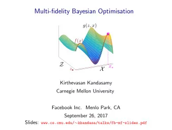
Multi-fidelity Optimisation with Continuous Approximations (Kandasamy et al. Arxiv 2017) Z X A fidelity space Z ⊂ R p and domain X ⊂ R d . 21/26

Multi-fidelity Optimisation with Continuous Approximations (Kandasamy et al. Arxiv 2017) g ( z, x ) Z X A fidelity space Z ⊂ R p and domain X ⊂ R d . g : Z × X → R . 21/26

Multi-fidelity Optimisation with Continuous Approximations (Kandasamy et al. Arxiv 2017) g ( z, x ) f ( x ) Z z • X A fidelity space Z ⊂ R p and domain X ⊂ R d . g : Z × X → R . We wish to optimise f ( x ) = g ( z • , x ) where z • ∈ Z . 21/26

Multi-fidelity Optimisation with Continuous Approximations (Kandasamy et al. Arxiv 2017) g ( z, x ) f ( x ) Z z • X A fidelity space Z ⊂ R p and domain X ⊂ R d . g : Z × X → R . We wish to optimise f ( x ) = g ( z • , x ) where z • ∈ Z . previous e.g.: Z = all ( N , T ) values, z • = [ N • , T • ]. 21/26

Multi-fidelity Optimisation with Continuous Approximations (Kandasamy et al. Arxiv 2017) g ( z, x ) f ( x ) Z z • X A fidelity space Z ⊂ R p and domain X ⊂ R d . g : Z × X → R . We wish to optimise f ( x ) = g ( z • , x ) where z • ∈ Z . previous e.g.: Z = all ( N , T ) values, z • = [ N • , T • ]. A cost function, λ : Z → R + . e.g.: λ ( z ) = λ ( N , T ) = O ( N 2 T ) 21/26

Multi-fidelity Optimisation with Continuous Approximations (Kandasamy et al. Arxiv 2017) g ( z, x ) f ( x ) Z x ⋆ z • X A fidelity space Z ⊂ R p and domain X ⊂ R d . g : Z × X → R . We wish to optimise f ( x ) = g ( z • , x ) where z • ∈ Z . previous e.g.: Z = all ( N , T ) values, z • = [ N • , T • ]. A cost function, λ : Z → R + . e.g.: λ ( z ) = λ ( N , T ) = O ( N 2 T ) x ⋆ = argmax x f ( x ). 21/26

Multi-fidelity Optimisation with Continuous Approximations (Kandasamy et al. Arxiv 2017) g ( z, x ) f ( x ) Z x ⋆ z • X A fidelity space Z ⊂ R p and domain X ⊂ R d . g : Z × X → R . We wish to optimise f ( x ) = g ( z • , x ) where z • ∈ Z . previous e.g.: Z = all ( N , T ) values, z • = [ N • , T • ]. A cost function, λ : Z → R + . e.g.: λ ( z ) = λ ( N , T ) = O ( N 2 T ) x ⋆ = argmax x f ( x ). Simple Regret: t : z t = z • f ( x t ) . S (Λ) = f ( x ⋆ ) − max 21/26

Multi-fidelity Optimisation with Continuous Approximations (Kandasamy et al. Arxiv 2017) g ( z, x ) g ∼ GP ( 0 , κ ), f ( x ) Z z • X 22/26

Multi-fidelity Optimisation with Continuous Approximations (Kandasamy et al. Arxiv 2017) g ( z, x ) κ : ( Z × X ) 2 → R . g ∼ GP ( 0 , κ ), f ( x ) Z z • X 22/26

Multi-fidelity Optimisation with Continuous Approximations (Kandasamy et al. Arxiv 2017) g ( z, x ) κ : ( Z × X ) 2 → R . g ∼ GP ( 0 , κ ), f ( x ) κ ([ z , x ] , [ z ′ , x ′ ]) = κ X ( x , x ′ ) · κ Z ( z , z ′ ) Z z • X 22/26

Multi-fidelity Optimisation with Continuous Approximations (Kandasamy et al. Arxiv 2017) g ( z, x ) κ : ( Z × X ) 2 → R . g ∼ GP ( 0 , κ ), f ( x ) κ ([ z , x ] , [ z ′ , x ′ ]) = κ X ( x , x ′ ) · κ Z ( z , z ′ ) Z z • X h = 0 . 05 h = 0 . 5 0 SE kernel: 22/26

Multi-fidelity Optimisation with Continuous Approximations (Kandasamy et al. Arxiv 2017) g ( z, x ) κ : ( Z × X ) 2 → R . g ∼ GP ( 0 , κ ), f ( x ) κ ([ z , x ] , [ z ′ , x ′ ]) = κ X ( x , x ′ ) · κ Z ( z , z ′ ) Z z • X Information Gap ξ : Z → R h = 0 . 05 h = 0 . 5 - measures the price (in information) for querying at z � = z • . 0 SE kernel: 22/26

Multi-fidelity Optimisation with Continuous Approximations (Kandasamy et al. Arxiv 2017) g ( z, x ) κ : ( Z × X ) 2 → R . g ∼ GP ( 0 , κ ), f ( x ) κ ([ z , x ] , [ z ′ , x ′ ]) = κ X ( x , x ′ ) · κ Z ( z , z ′ ) Z z • X Information Gap ξ : Z → R h = 0 . 05 h = 0 . 5 - measures the price (in information) for querying at z � = z • . 0 � z − z • � SE kernel: ξ ( z ) � . h 22/26