Background Subtraction Birgi Tamersoy The University of Texas at - PowerPoint PPT Presentation
Background Subtraction Birgi Tamersoy The University of Texas at Austin September 29 th , 2009 Background Subtraction Given an image (mostly likely to be a video frame), we want to identify the foreground objects in that image!
Background Subtraction Birgi Tamersoy The University of Texas at Austin September 29 th , 2009
Background Subtraction ◮ Given an image (mostly likely to be a video frame), we want to identify the foreground objects in that image! ⇒ Motivation ◮ In most cases, objects are of interest, not the scene. ◮ Makes our life easier: less processing costs, and less room for error.
Widely Used! ◮ Traffic monitoring (counting vehicles, detecting & tracking vehicles), ◮ Human action recognition (run, walk, jump, squat, . . . ), ◮ Human-computer interaction (“human interface”), ◮ Object tracking (watched tennis lately?!?), ◮ And in many other cool applications of computer vision such as digital forensics. http://www.crime-scene-investigator.net/ DigitalRecording.html
Requirements ◮ A reliable and robust background subtraction algorithm should handle: ◮ Sudden or gradual illumination changes, ◮ High frequency, repetitive motion in the background (such as tree leaves, flags, waves, . . . ), and ◮ Long-term scene changes (a car is parked for a month).
Simple Approach Image at time t : Background at time t : I ( x , y , t ) B ( x , y , t ) ⇓ ⇓ | − | > Th 1. Estimate the background for time t . 2. Subtract the estimated background from the input frame. 3. Apply a threshold, Th , to the absolute difference to get the foreground mask . But, how can we estimate the background?
Frame Differencing ◮ Background is estimated to be the previous frame. Background subtraction equation then becomes: B ( x , y , t ) = I ( x , y , t − 1) ⇓ | I ( x , y , t ) − I ( x , y , t − 1) | > Th ◮ Depending on the object structure, speed, frame rate and global threshold, this approach may or may not be useful (usually not ). | − | > Th
Frame Differencing Th = 25 Th = 50 Th = 100 Th = 200
Mean Filter ◮ In this case the background is the mean of the previous n frames: B ( x , y , t ) = 1 � n − 1 i =0 I ( x , y , t − i ) n ⇓ | I ( x , y , t ) − 1 � n − 1 i =0 I ( x , y , t − i ) | > Th n ◮ For n = 10: Estimated Background Foreground Mask
Mean Filter ◮ For n = 20: Estimated Background Foreground Mask ◮ For n = 50: Estimated Background Foreground Mask
Median Filter ◮ Assuming that the background is more likely to appear in a scene, we can use the median of the previous n frames as the background model: B ( x , y , t ) = median { I ( x , y , t − i ) } ⇓ | I ( x , y , t ) − median { I ( x , y , t − i ) }| > Th where i ∈ { 0 , . . . , n − 1 } . ◮ For n = 10: Estimated Background Foreground Mask
Median Filter ◮ For n = 20: Estimated Background Foreground Mask ◮ For n = 50: Estimated Background Foreground Mask
Advantages vs. Shortcomings Advantages: ◮ Extremely easy to implement and use! ◮ All pretty fast. ◮ Corresponding background models are not constant, they change over time. Disadvantages: ◮ Accuracy of frame differencing depends on object speed and frame rate! ◮ Mean and median background models have relatively high memory requirements. ◮ In case of the mean background model, this can be handled by a running average : B ( x , y , t ) = t − 1 t B ( x , y , t − 1) + 1 t I ( x , y , t ) or more generally: B ( x , y , t ) = (1 − α ) B ( x , y , t − 1) + α I ( x , y , t ) where α is the learning rate.
Advantages vs. Shortcomings Disadvantages: ◮ There is another major problem with these simple approaches: | I ( x , y , t ) − B ( x , y , t ) | > Th 1. There is one global threshold, Th , for all pixels in the image. 2. And even a bigger problem: this threshold is not a function of t . ◮ So, these approaches will not give good results in the following conditions: ◮ if the background is bimodal, ◮ if the scene contains many, slowly moving objects (mean & median), ◮ if the objects are fast and frame rate is slow (frame differencing), ◮ and if general lighting conditions in the scene change with time!
“The Paper” on Background Subtraction Adaptive Background Mixture Models for Real-Time Tracking Chris Stauffer & W.E.L. Grimson
Motivation ◮ A robust background subtraction algorithm should handle: lighting changes , repetitive motions from clutter and long-term scene changes . Stauffer & Grimson
A Quick Reminder: Normal (Gaussian) Distribution ◮ Univariate: 2 πσ 2 e − ( x − µ )2 N ( x | µ, σ 2 ) = 1 √ 2 σ 2 ◮ Multivariate: 2 ( x − µ ) T Σ − 1 ( x − µ ) | Σ | 1 / 2 e − 1 1 1 N ( x | µ, Σ ) = (2 π ) D / 2 http://en.wikipedia.org/wiki/Normal distribution
Algorithm Overview ◮ The values of a particular pixel is modeled as a mixture of adaptive Gaussians. ◮ Why mixture? Multiple surfaces appear in a pixel. ◮ Why adaptive? Lighting conditions change. ◮ At each iteration Gaussians are evaluated using a simple heuristic to determine which ones are mostly likely to correspond to the background. ◮ Pixels that do not match with the “background Gaussians” are classified as foreground. ◮ Foreground pixels are grouped using 2D connected component analysis.
Online Mixture Model ◮ At any time t , what is known about a particular pixel, ( x 0 , y 0 ), is its history: { X 1 , . . . , X t } = { I ( x 0 , y 0 , i ) : 1 ≤ i ≤ t } ◮ This history is modeled by a mixture of K Gaussian distributions: P ( X t ) = � K i =1 ω i , t ∗ N ( X t | µ i , t , Σ i , t ) where 2 ( X t − µ i , t ) T Σ − 1 | Σ i , t | 1 / 2 e − 1 1 1 i , t ( X t − µ i , t ) N ( X t | µ it , Σ i , t ) = (2 π ) D / 2 What is the dimensionality of the Gaussian?
Online Mixture Model ◮ If we assume gray scale images and set K = 5, history of a pixel will be something like this:
Model Adaptation ◮ An on-line K-means approximation is used to update the Gaussians. ◮ If a new pixel value, X t +1 , can be matched to one of the existing Gaussians (within 2 . 5 σ ), that Gaussian’s µ i , t +1 and σ 2 i , t +1 are updated as follows: µ i , t +1 = (1 − ρ ) µ i , t + ρ X t +1 and σ 2 i , t +1 = (1 − ρ ) σ 2 i , t + ρ ( X t +1 − µ i , t +1 ) 2 where ρ = α N ( X t +1 | µ i , t , σ 2 i , t ) and α is a learning rate. ◮ Prior weights of all Gaussians are adjusted as follows: ω i , t +1 = (1 − α ) ω i , t + α ( M i , t +1 ) where M i , t +1 = 1 for the matching Gaussian and M i , t +1 = 0 for all the others.
Model Adaptation ◮ If X t +1 do not match to any of the K existing Gaussians, the least probably distribution is replaced with a new one. ◮ Warning!!! “Least probably” in the ω/σ sense (will be explained). ◮ New distribution has µ t +1 = X t +1 , a high variance and a low prior weight.
Background Model Estimation ◮ Heuristic: the Gaussians with the most supporting evidence and least variance should correspond to the background (Why?). ◮ The Gaussians are ordered by the value of ω/σ (high support & less variance will give a high value). ◮ Then simply the first B distributions are chosen as the background model: B = argmin b ( � b i =1 ω i > T ) where T is minimum portion of the image which is expected to be background.
Background Model Estimation ◮ After background model estimation red distributions become the background model and black distributions are considered to be foreground.
Advantages vs. Shortcomings Advantages: ◮ A different “threshold” is selected for each pixel. ◮ These pixel-wise “thresholds” are adapting by time. ◮ Objects are allowed to become part of the background without destroying the existing background model. ◮ Provides fast recovery. Disadvantages: ◮ Cannot deal with sudden, drastic lighting changes! ◮ Initializing the Gaussians is important (median filtering). ◮ There are relatively many parameters, and they should be selected intelligently.
Does it get more complicated? ◮ Chen & Aggarwal: The likelihood of a pixel being covered or uncovered is decided by the relative coordinates of optical flow vector vertices in its neighborhood. ◮ Oliver et al.: “Eigenbackgrounds” and its variations. ◮ Seki et al.: Image variations at neighboring image blocks have strong correlation.
Example: A Simple & Effective Background Subtraction Approach Adaptive Background 3D Connected Mixture Model + Component Analysis (3 rd dimension: time ) (Stauffer & Grimson) ◮ 3D connected component analysis incorporates both spatial and temporal information to the background model (by Goo et al.)!
Video Examples
Summary ◮ Simple background subtraction approaches such as frame differencing , mean and median filtering, are pretty fast. ◮ However, their global, constant thresholds make them insufficient for challenging real-world problems. ◮ Adaptive background mixture model approach can handle challenging situations: such as bimodal backgrounds, long-term scene changes and repetitive motions in the clutter. ◮ Adaptive background mixture model can further be improved by incorporating temporal information , or using some regional background subtraction approaches in conjunction with it .
Recommend
More recommend
Explore More Topics
Stay informed with curated content and fresh updates.
