Background Models and Languages for The modelling of chemical - PDF document

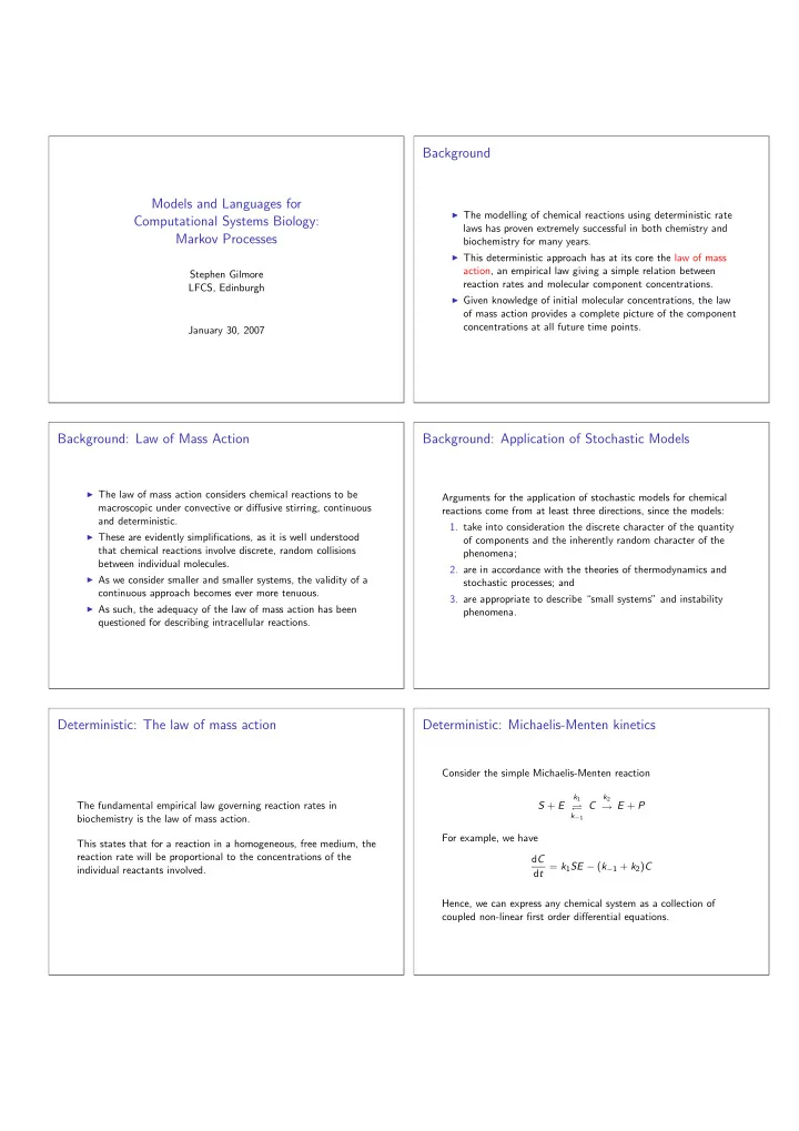
Background Models and Languages for ◮ The modelling of chemical reactions using deterministic rate Computational Systems Biology: laws has proven extremely successful in both chemistry and Markov Processes biochemistry for many years. ◮ This deterministic approach has at its core the law of mass action, an empirical law giving a simple relation between Stephen Gilmore reaction rates and molecular component concentrations. LFCS, Edinburgh ◮ Given knowledge of initial molecular concentrations, the law of mass action provides a complete picture of the component concentrations at all future time points. January 30, 2007 Background: Law of Mass Action Background: Application of Stochastic Models ◮ The law of mass action considers chemical reactions to be Arguments for the application of stochastic models for chemical macroscopic under convective or diffusive stirring, continuous reactions come from at least three directions, since the models: and deterministic. 1. take into consideration the discrete character of the quantity ◮ These are evidently simplifications, as it is well understood of components and the inherently random character of the that chemical reactions involve discrete, random collisions phenomena; between individual molecules. 2. are in accordance with the theories of thermodynamics and ◮ As we consider smaller and smaller systems, the validity of a stochastic processes; and continuous approach becomes ever more tenuous. 3. are appropriate to describe “small systems” and instability ◮ As such, the adequacy of the law of mass action has been phenomena. questioned for describing intracellular reactions. Deterministic: The law of mass action Deterministic: Michaelis-Menten kinetics Consider the simple Michaelis-Menten reaction k 1 k 2 The fundamental empirical law governing reaction rates in S + E C → E + P ⇋ k − 1 biochemistry is the law of mass action. For example, we have This states that for a reaction in a homogeneous, free medium, the reaction rate will be proportional to the concentrations of the d C d t = k 1 SE − ( k − 1 + k 2 ) C individual reactants involved. Hence, we can express any chemical system as a collection of coupled non-linear first order differential equations.

Stochastic: Random processes Stochastic: Predictability of macroscopic states ◮ In macroscopic systems, with a large number of interacting ◮ Whereas the deterministic approach outlined above is molecules, the randomness of this behaviour averages out so essentially an empirical law, derived from in vitro experiments, that the overall macroscopic state of the system becomes the stochastic approach is far more physically rigorous. highly predictable. ◮ Fundamental to the principle of stochastic modelling is the ◮ It is this property of large scale random systems that enables a idea that molecular reactions are essentially random processes; deterministic approach to be adopted; however, the validity of it is impossible to say with complete certainty the time at this assumption becomes strained in in vivo conditions as we which the next reaction within a volume will occur. examine small-scale cellular reaction environments with limited reactant populations. Random experiments and events Random variables ◮ To apply probability theory to the process under study, we view it as a random experiment. We are interested in the dynamics of a system as events happen over time. A function which associates a (real-valued) number ◮ The sample space of a random experiment is the set of all with the outcome of an experiment is known as a random variable. individual outcomes of the experiment. Formally, a random variable X is a real-valued function defined on ◮ These individual outcomes are also called sample points or a sample space Ω. elementary events. ◮ An event is a subset of a sample space. Measurable functions Distribution function If X is a random variable, and x is a real number, we write X ≤ x for the event For each random variable X we define its distribution function F { ω : ω ∈ Ω and X ( ω ) ≤ x } for each real x by F ( x ) = Pr[ X ≤ x ] and we write X = x for the event We associate another function p ( · ), called the probability mass { ω : ω ∈ Ω and X ( ω ) = x } function of X (pmf), for each real x : Another property required of a random variable is that the set p ( x ) = Pr[ X = x ] X ≤ x is an event for each real x . This is necessary so that probability calculations can be made. A function having this property is said to be a measurable function or measurable in the Borel sense.

Continuous random variables Exponential random variables, distribution function The random variable X is said to be an exponential random A random variable X is continuous if p ( x ) = 0 for all real x . variable with parameter λ ( λ > 0) or to have an exponential distribution with parameter λ if it has the distribution function (If X is a continuous random variable, then X can assume � 1 − e − λ x infinitely many values, and so it is reasonable that the probability for x > 0 of its assuming any specific value we choose beforehand is zero.) F ( x ) = 0 for x ≤ 0 The distribution function for a continuous random variable is a Some authors call this distribution the negative exponential continuous function in the usual sense. distribution. Exponential random variables, density function Notation: indicator functions We sometimes instead see functions such as � λ e − λ x if x > 0 The density function f = dF / dx is given by f ( x ) = 0 if x ≤ 0 � λ e − λ x if x > 0 f ( x ) = written as 0 if x ≤ 0 f ( x ) = λ e − λ x 1 x > 0 The function 1 x > 0 is an indicator function (used to code the conditional part of the definition). A Computer Scientist would write this as if x>0 then 1 else 0 or (x > 0) ? 1 : 0 Mean, or expected value Mean, or expected value, of the exponential distribution If X is a continuous random variable with density function f ( · ), we Suppose X has an exponential distribution with parameter λ > 0. define the mean or expected value of X , µ = E [ X ] by Then � ∞ x λ e − λ x dx = 1 � ∞ µ = E [ X ] = µ = E [ X ] = xf ( x ) dx λ −∞ −∞

Exponential inter-event time distribution Memoryless property of the exponential distribution The time interval between successive events can also be deduced. Let F ( t ) be the distribution function of T , the time between events. Consider Pr( T > t ) = 1 − F ( t ): The memoryless property of the exponential distribution is so Pr( T > t ) = Pr(No events in an interval of length t ) called because the time to the next event is independent of when the last event occurred. = 1 − F ( t ) 1 − (1 − e − λ t ) = e − λ t = Memoryless property of the exponential distribution Markov processes A finite-state stochastic process X ( t ), with exponentially-distributed transitions between states is a Markov Suppose that the last event was at time 0. What is the probability process. This can be described by the state-transition matrix, Q Q . Q that the next event will be after t + s , given that time t has elapsed since the last event, and no events have occurred? A stationary or equilibrium probability distribution, π ( · ), exists for every time-homogeneous irreducible Markov process whose states Pr( T > t + s and T > t ) Pr( T > t + s | T > t ) = are all positive-recurrent. Pr( T > t ) e − λ ( t + s ) This distribution is found by solving the global balance equation = e − λ t e − λ s = π Q Q Q = 0 subject to the normalisation condition This value is independent of t (and so the time already spent has not been remembered). � π ( C i ) = 1 . Continuous-Time Markov Chains (CTMCs) Markov processes in Systems Biology A Markov process with discrete state space and discrete index set Markov processes in systems biology are sometimes generated from is called a Markov chain. The future behaviour of a Markov chain a high-level language description in a language with an interleaving depends only on its current state, and not on how that state was semantics. reached. This is the Markov, or memoryless, property. Other modelling formalisms based on CTMCs are also based on an Pr( X ( t n +1 ) = x n +1 | X ( t n ) = x n , . . . , X ( t 0 ) = x 0 ) interleaving semantics (e.g. Generalised Stochastic Petri nets). = Pr( X ( t n +1 ) = x n +1 | X ( t n ) = x n )