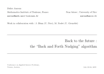
Back to the future : the Back and Forth Nudging Scaling Up and - PowerPoint PPT Presentation

Jacques Blum Didier Auroux University of Nice Sophia Antipolis University of Toulouse jblum@unice.fr auroux@math.univ-toulouse.fr Back to the future : the Back and Forth Nudging Scaling Up and Modeling for Transport and Flow in Porous Media Dubrovnik, Croatia October 13-16 2008

Motivations Motivation : Identify the initial condition in a geophysical system Fundamental for a chaotic system (Lorenz, atmosphere, ocean, . . .) Difficulty : These systems are generally irreversible. Comparison with 4D-VAR : Optimal control method minimizing the qua- dratic difference between model and observations. Dubrovnik, October 13-16 2008 1/26

Forward nudging Let us consider a model governed by a system of ODE : dX dt = F ( X ) , 0 < t < T, with an initial condition X (0) = x 0 . X obs ( t ) : observations of the system C : observation operator. dX  dt = F ( X )+ K ( X obs − C ( X )) , 0 < t < T,    X (0) = x 0 ,  where K is the nudging (or gain) matrix. In the linear case (where F is a matrix), the forward nudging is called Luen- berger or asymptotic observer. Dubrovnik, October 13-16 2008 2/26

Direct Nudging – Meteorology : Hoke-Anthes (1976) – Oceanography ( QG model) : Verron-Holland (1989) – Atmosphere (meso-scale) : Stauffer-Seaman (1990) – Optimal determination of the nudging coeffcients : Zou-Navon-Le Dimet (1992), Stauffer-Bao (1993), Vidard-Le Dimet-Piacentini (2003) Dubrovnik, October 13-16 2008 3/26

Direct Nudging : linear case Luenberger observer, or asymptotic observer (Luenberger, 1966) dX  dt = FX + K ( X obs − CX ) ,    d ˆ X  dt = F ˆ X obs = C ˆ  X, X.  d dt ( X − ˆ X ) = ( F − KC )( X − ˆ X ) If F − KC is a Hurwitz matrix, i.e. its spectrum is strictly included in the half-plane { λ ∈ C ; Re ( λ ) < 0 } , then X → ˆ X when t → + ∞ . Dubrovnik, October 13-16 2008 4/26

Backward nudging Backward model : (Auroux, 2003) d ˜  X dt = F ( ˜ X ) , T > t > 0 ,   ˜  X ( T ) = ˜ x T .  If we apply nudging to this backward model : d ˜  X dt = F ( ˜ X ) − K ′ ( X obs − C ( ˜ X )) , T > t > 0 ,   ˜  X ( T ) = ˜ x T .  t ′ = T − t : d ˜  X 0 < t ′ < T, dt ′ = − F ( ˜ X )+ K ′ ( X obs − C ( ˜ X )) ,   ˜  X (0) = ˜ x T .  In the linear case, − F − K ′ C must be a Hurwitz matrix. Dubrovnik, October 13-16 2008 5/26

BFN : Back and Forth Nudging algorithm Iterative algorithm (forward and backward resolutions) : ˜ X 0 (0) = ˜ x 0 (first guess)  dX k = F ( X k )+ K ( X obs − C ( X k ))   dt X k (0) = ˜ X k − 1 (0)   d ˜  X k = F ( ˜ X k ) − K ′ ( X obs − C ( ˜ X k ))   dt ˜  X k ( T ) = X k ( T )  Dubrovnik, October 13-16 2008 6/26

e ( C = Id , K = K ′ ) Cas simplifi´ Convergence in a linear case , with full observations : D. Auroux, J. Blum, Back and forth nudging algorithm for data assimilation problems, C. R. Acad. Sci. Ser. I , 340 , pp. 873–878, 2005. k → + ∞ X k (0) = X ∞ (0) lim I − e − 2 KT � − 1 � T e − ( K + F ) s + e − 2 KT e ( K − F ) s � � � = KX obs ( s ) ds. 0 � t k → + ∞ X k ( t ) = X ∞ ( t ) = e − ( K − F ) t e ( K − F ) s KX obs ( s ) ds + e − ( K − F ) t X ∞ (0) . lim 0 If X obs ( t ) = e F t x 0 , then, if K and F commute, X ∞ ( t ) = X obs ( t ) , ∀ t ∈ [0; T ] . Dubrovnik, October 13-16 2008 7/26

Choice of the direct nudging matrix K Implicit discretization of the direct model equation with nudging : X n +1 − X n = FX n +1 + K ( X obs − CX n +1 ) . ∆ t Variational interpretation : direct nudging is a compromise between the mini- mization of the energy of the system and the quadratic distance to the obser- vations : � 1 2 � X − X n , X − X n � − ∆ t 2 � FX, X � + ∆ t � 2 � R − 1 ( X obs − CX ) , X obs − CX � min , X by choosing K = C T R − 1 where R is the covariance matrix of the errors of observation. Auroux-Blum, Nonlinear Processes in Geophysics (2008) Dubrovnik, October 13-16 2008 8/26

Choice of the backward nudging matrix K ′ The feedback term has a double role : • stabilization of the backward resolution of the model (irreversible system) • feedback to the observations If the system is observable, i.e. rank [ C, CF, . . . , CF N − 1 ] = N , then there exists a matrix K ′ such that − F − K ′ C is a Hurwitz matrix (pole assignment method). In practice, K ′ = k ′ C T and k ′ can be chosen as being the smallest value making the backward numerical resolution stable. Dubrovnik, October 13-16 2008 9/26

4D-VAR x b Observations x 0 dx  dt = F ( x ) ,    x (0) = x 0 ,  t x obs ( t ) : observations of the system, C : observation operator, and R : covariance matrices of background and observation errors B respectively. 1 2( x 0 − x b ) T B − 1 ( x 0 − x b ) J ( x 0 ) = � T 1 [ x obs ( t ) − C ( x ( t ))] T R − 1 [ x obs ( t ) − C ( x ( t ))] dt + 2 0 Dubrovnik, October 13-16 2008 10/26

Optimality System Optimization under constraints : � T � � p, dx L ( x 0 , x, p ) = J ( x 0 ) + dt − F ( x ) dt 0 dx  dt = F ( x )  Direct model : x (0) = x 0  � T  � ∂F − dp p + C T R − 1 [ x obs ( t ) − C ( x ( t ))]  dt =  Adjoint model : ∂x  p ( T ) = 0  Gradient of the cost-function : ∂J = B − 1 ( x 0 − x b ) − p (0) = 0 ∂x 0 Le Dimet - Talagrand (86) Dubrovnik, October 13-16 2008 11/26

N UMERICAL R ESULTS L ORENZ E QUATION Dubrovnik, October 13-16 2008 12/26

Lorenz’ equations 50 dx  40 dt = 10 ( y − x ) ,    30   z(t)   dy  20 dt = 28 x − y − xz, 10     dt = − 8 dz  0  3 z + xy.  30  20 20 10 10 0 0 −10 −10 −20 −30 −20 y(t) x(t) – Assimilation period : [0; 3], forecast : [3; 6]. – Time step : 0 . 001. – 31 observations (every 100 time steps). Dubrovnik, October 13-16 2008 13/26

Convergence 10 x 8 y z 6 X k (0) − X true 4 2 0 −2 −4 0 5 10 15 20 25 30 35 40 45 BFN iterations Fig. 1 – Difference between the k th iterate X k (0) and the exact initial condition x true for the 3 variables versus the number of BFN iterations. Dubrovnik, October 13-16 2008 14/26

Convergence 30 20 x y 10 z X k+1 (0) − X k (0) 0 −10 −20 −30 −40 −50 −60 0 5 10 15 20 25 30 35 40 BFN iterations Fig. 2 – Difference between two consecutive BFN iterates for the 3 variables versus the number of BFN iterations. Dubrovnik, October 13-16 2008 15/26

Convergence 2500 x y 2000 z − X obs || 2 1500 ||X k 1000 500 0 0 5 10 15 20 25 30 35 40 BFN iterations Fig. 3 – RMS difference between the observations and the BFN identified trajectory versus the BFN iterations. Dubrovnik, October 13-16 2008 16/26

Comparison with 4D-VAR 20 True BFN 15 4D−VAR 10 5 x 0 −5 −10 −15 −20 0 1 2 3 4 5 6 Time Fig. 4 – Evolution in time of the reference trajectory (plain line), and of the trajectories identified by the 4D-VAR (dashed line) and the BFN (dash-dotted line) algorithms, in the case of perfect observations and for the first Lorenz variable x . Dubrovnik, October 13-16 2008 17/26

Comparison with 4D-VAR 20 True Perturbed 15 BFN 4D−VAR 10 5 x 0 −5 −10 −15 −20 0 1 2 3 4 5 6 Time Fig. 5 – Evolution in time of the reference trajectories (plain line), and of the trajectories identified by the 4D-VAR (dashed line) and the BFN (dash-dotted line) algorithms, in the case of noised observations (with a 10% gaussian blank noise) and for the first Lorenz variable x . Dubrovnik, October 13-16 2008 18/26

N UMERICAL R ESULTS B URGERS E QUATION Dubrovnik, October 13-16 2008 19/26

1D viscous Burgers’ equation ∂X 2 ∂s − ν ∂ 2 X ∂X ∂t + 1 ∂s 2 = 0 , 2 where X is the state variable, s represents the distance in meters around the 45 o N constant-latitude circle and t is the time. The period of the domain is roughly 28 . 3 × 10 6 m . The diffusion coefficient ν is set to 10 5 m 2 .s − 1 . The time step is one hour, and the assimilation period is roughly one month (700 time steps). Data : every 10 time steps (10 hours), every 5 gridpoints, 5% RMS blank gaussian error. Dubrovnik, October 13-16 2008 20/26

Convergence 0.7 0.6 0.5 RMS relative difference 0.4 0.3 0.2 0.1 0 1 2 3 4 5 6 7 BFN iterations Fig. 6 – RMS relative difference between two consecutive iterates of the BFN algorithm versus the number of iterations. Dubrovnik, October 13-16 2008 21/26

Convergence 1 0.8 0.9 0.7 0.8 0.6 0.7 RMS relative error RMS relative error 0.5 0.6 0.4 0.5 0.3 0.4 0.2 0.3 0.1 0.2 0.1 0 0 1 2 3 4 5 6 7 8 0 1 2 3 4 5 6 7 8 BFN iterations BFN iterations Fig. 7 – RMS relative difference between the BFN iterates and the exact solution versus the number of iterations, at time t = 0 (a) and at time t = T (b). Dubrovnik, October 13-16 2008 22/26