Axial vectors and transversal short-distance constraints Martin - PowerPoint PPT Presentation
Axial vectors and transversal short-distance constraints Martin Hoferichter Institute for Nuclear Theory University of Washington Third Plenary Workshop of the Muon g 2 Theory Initiative INT Workshop on Hadronic contributions to ( g 2 )
Axial vectors and transversal short-distance constraints Martin Hoferichter Institute for Nuclear Theory University of Washington Third Plenary Workshop of the Muon g − 2 Theory Initiative INT Workshop on Hadronic contributions to ( g − 2 ) µ Seattle, September 12, 2019 M. Hoferichter (Institute for Nuclear Theory) Axials and transversal SDCs Seattle, September 12, 2019 1
Motivation Short-distance constraints for mixed region: OPE, VVA anomaly Melnikov, Vainshtein 2004 Mapping onto BTT see my talk from Mainz meeting Longitudinal constraints: ˆ Π 1–3 , related to pseudoscalar poles see talk by L. Laub Transversal constraints: all other ˆ Π i Status of the axial vectors a 1 ( 1260 ) , f 1 ( 1285 ) , f ′ 1 ( 1420 ) a 1 + f 1 + f ′ MV = 22 × 10 − 11 (used to saturate transversal SDCs) � Large in MV: a 1 µ � Jegerlehner 2017 : MV model violates Landau–Yang theorem a 1 + f 1 + f ′ 1 � J = 8 × 10 − 11 ֒ → introduces antisymmetrization by hand ⇒ a µ � f 1 + f ′ � PV = 6 × 10 − 11 1 Pauk, Vanderhaeghen 2014 : Lagrangian model, a µ � This talk: BTT decomposition for axials Mapping of MV model onto BTT ֒ → clarify Landau–Yang, explain why MV number is so large M. Hoferichter (Institute for Nuclear Theory) Axials and transversal SDCs Seattle, September 12, 2019 2
Axial vectors: matrix element Decomposition of A → γ ∗ γ ∗ amplitude � γ ∗ ( q 1 , λ 1 ) γ ∗ ( q 2 , λ 2 ) | A ( p , λ A ) � = i ( 2 π ) 4 δ ( 4 ) ( q 1 + q 2 − p ) e 2 ǫ λ 1 ∗ ǫ λ 2 ∗ ǫ λ A α M µνα ( q 1 , q 2 ) µ ν 3 i M µνα ( q 1 , q 2 ) = � T µνα F i ( q 2 1 , q 2 2 ) m 2 i A i = 1 → three form factors F i ( q 2 1 , q 2 ֒ 2 ) Lorentz structures from BTT recipe T µνα = ǫ µνβγ q 1 β q 2 γ ( q α 1 − q α 2 ) 1 T µνα = ǫ ανβγ q 1 β q 2 γ q µ 1 + ǫ αµνβ q 2 β q 2 2 1 T µνα = ǫ αµβγ q 1 β q 2 γ q ν 2 + ǫ αµνβ q 1 β q 2 2 3 Crossing properties � = − T µνα � = − T µνα � T µνα � T µνα C 12 C 12 1 1 2 3 F 1 ( q 2 1 , q 2 2 ) = −F 1 ( q 2 2 , q 2 F 2 ( q 2 1 , q 2 2 ) = −F 3 ( q 2 2 , q 2 1 ) 1 ) F 1 ( 0 , 0 ) = 0 F 2 ( 0 , 0 ) = −F 3 ( 0 , 0 ) M. Hoferichter (Institute for Nuclear Theory) Axials and transversal SDCs Seattle, September 12, 2019 3
Axial vectors: phenomenology Landau–Yang in action: 2 ) = λ ( m 2 A , q 2 1 , q 2 2 ) − q 2 1 ( m 2 A − q 2 1 + q 2 2 ) − q 2 2 ( m 2 A + q 2 1 − q 2 2 ) 2 ) 2 ) H ++ ( q 2 1 , q 2 F 1 ( q 2 1 , q 2 F 2 ( q 2 1 , q 2 F 3 ( q 2 1 , q 2 2 ) 2 m 3 2 m 3 2 m 3 A A A q 2 1 , q 2 → 0 for 2 → 0 Equivalent two-photon photon width m 2 L γ T ) = πα 2 m A 1 � 2 ˜ A � � Γ γγ = lim 2 Γ( A → γ ∗ � F 2 ( 0 , 0 ) q 2 12 q 2 1 → 0 1 Experimental input from e + e − → e + e − f 1 ( ′ ) L3 2002, 2007 ˜ ˜ Γ γγ ( f 1 ) = 3 . 5 ( 8 ) keV Γ γγ ( f ′ 1 ) BR ( f ′ 1 → KK π ) = 3 . 2 ( 9 ) keV Λ D ( f ′ Λ D ( f 1 ) = 1 . 04 ( 8 ) GeV 1 ) = 0 . 93 ( 8 ) GeV assuming Schuler et al. 1998 � − 2 F 2 ( − Q 2 , 0 ) 1 + Q 2 � F 1 ( − Q 2 , 0 ) = 0 = Λ 2 F 2 ( 0 , 0 ) D M. Hoferichter (Institute for Nuclear Theory) Axials and transversal SDCs Seattle, September 12, 2019 4
Axial vectors: mixing and SU ( 3 ) Mixing of f 1 and f ′ 1 f 0 f 1 cos θ A sin θ A = 1 f 8 f ′ − sin θ A cos θ A 1 1 Mixing angle ˜ = m f 1 Γ γγ ( f 1 ) θ 0 = arcsin 1 cot 2 ( θ A − θ 0 ) θ A = 62 ( 5 ) ◦ ˜ Γ γγ ( f ′ 1 ) m f ′ 3 1 Assume SU ( 3 ) symmetry for axial nonet φ √ √ Tr ( Q 2 φ ) = 1 � � 6 f 0 3 f 8 3 a 1 + 2 1 + 1 9 ˜ ˜ Γ γγ ( f ′ Γ γγ ( f 1 ) m a 1 1 ) m a 1 ˜ Γ γγ ( a 1 ) = = = 2 . 1 keV 3 cos 2 ( θ A − θ 0 ) 3 sin 2 ( θ A − θ 0 ) m f 1 m f ′ 1 M. Hoferichter (Institute for Nuclear Theory) Axials and transversal SDCs Seattle, September 12, 2019 5
BTT projection of MV constraints MV constraint for q 2 3 ≪ q 2 1 ∼ q 2 2 , ˆ q = ( q 1 − q 2 ) / 2 ˆ Π 1 = 2 w L ( q 2 q 2 ) 3 ) f (ˆ Π 5 = ˆ ˆ Π 6 = w T ( q 2 q 2 ) 3 ) f (ˆ 1 Π 10 = ˆ ˆ Π 14 = − ˆ Π 17 = − ˆ Π 39 = − ˆ Π 50 = − ˆ w T ( q 2 q 2 ) 3 ) f (ˆ Π 51 = q 1 · q 2 ˆ Π i = 0 i ∈ { 2 , 3 , 4 , 7 , 8 , 9 , 11 , 13 , 16 , 54 } where 1 1 C 3 = 1 1 2 � q 2 ) = − C 2 f (ˆ a = − C 8 = √ C 0 = √ 2 π 2 ˆ q 2 18 π 2 ˆ q 2 6 6 3 3 6 a = 0 , 3 , 8 Non-renormalization theorems and anomaly condition in chiral limit Vainshtein 2003, Czarnecki et al. 2003, Knecht et al. 2004, . . . w L ( q 2 ) = 2 w T ( q 2 ) = 6 q 2 Transversal relation receives non-perturbative corrections M. Hoferichter (Institute for Nuclear Theory) Axials and transversal SDCs Seattle, September 12, 2019 6
Matching onto MV model Saturate transversal constraint from axial exchange, drop longitudinal amplitudes q 2 ˆ 8 1 � � C 2 a w T ( q 2 φ A ( q 2 1 , q 2 2 ) F A 2 ( q 2 3 ) = 3 , 0 ) q 2 ˆ m 4 q 2 3 − m 2 A A a = 0 , 3 , 8 A = a 1 , f 1 , f ′ 1 Λ 4 φ A ( q 2 1 , q 2 2 ) = F A 2 ( q 2 1 , q 2 2 ) + F A 2 ( q 2 2 , q 2 1 ) = 2 F A A 2 ( 0 , 0 ) (Λ 2 A − q 2 1 )(Λ 2 A − q 2 2 ) Conclusions F 2 ( q 2 1 , q 2 2 ) = −F 3 ( q 2 2 , q 2 1 ) , but φ ( q 2 1 , q 2 2 ) indeed symmetric ֒ → additional antisymmetrization in Jegerlehner 2017 incorrect q 4 and F 2 ( q 2 Scaling matches for φ ( q 2 1 , q 2 2 ) ∼ 1 / ˆ 3 , 0 ) → F 2 ( 0 , 0 ) � Λ A ˜ � 4 Λ A = 0 . 77 GeV Γ γγ ( A ) ? � C 2 � 1 = 9 = 9 = 0 . 04 a πα 2 m A m A a = 0 , 3 , 8 A = a 1 , f 1 , f ′ 1 ֒ → axial vectors with VMD not enough to saturate constraint , need Λ A ∼ 1 . 7 GeV M. Hoferichter (Institute for Nuclear Theory) Axials and transversal SDCs Seattle, September 12, 2019 7
Consequences Original MV estimates for different mixing scenarios | MV = ( 5 . 7 + 15 . 6 + 0 . 8 ) × 10 − 11 = 22 × 10 − 11 a ideal µ | MV = ( 5 . 7 + 1 . 9 + 9 . 7 ) × 10 − 11 = 17 × 10 − 11 a octet/singlet µ Comparison in BTT Model only well defined in OPE limit, need to pick kinematics in ˆ Π 4–6 ֒ → key difference to pseudoscalar poles, which are already the proper residues Axial propagators modified to enforce w L ( q 2 ) = 2 w T ( q 2 ) at O ( 1 / q 4 ) ֒ → depends on mixing scheme not only for axials, but also for pseudoscalars For VMD find similar numbers as MV Increasing the VMD scale to correct ˜ Γ γγ decreases a axials by about a factor 3 µ M. Hoferichter (Institute for Nuclear Theory) Axials and transversal SDCs Seattle, September 12, 2019 8
Conclusions MV model does not violate the Landau–Yang theorem , the critical combination of axial form factors is indeed symmetric MV model implies significantly too large two-photon widths ˜ Γ γγ Changing the VMD scale in the model to fix the widths decreases a axials µ All existing estimates for axial vectors are based on Lagrangian assumptions ֒ → need to isolate the residues and study the sum rules Transversal OPE constraint will be helpful for the mixed regions , just as the longitudinal one for the pseudoscalars M. Hoferichter (Institute for Nuclear Theory) Axials and transversal SDCs Seattle, September 12, 2019 9
Outlook: matching to the quark loop 20 Λ = ∞ Red: longitudinal ˆ Π 1–3 , blue: transversal, Λ = 1 GeV 15 Λ = 1 . 35 GeV a µ × 10 11 black: all 10 Integration region θ ( Q 1 − Q min ) θ ( Q 2 − Q min ) θ ( Q 3 − Q min ) 5 Q 2 3 + θ ( Q 1 − Q min ) θ ( Q 2 − Q min ) θ ( Q min − Q 3 ) Q 2 3 + Λ 2 0 1 1.5 2 2.5 3 + crossed Q min [GeV] Regge implementation of longitudinal SDCs see talk by L. Laub µ + ∆ a η ′ ∆ a η ∼ C 2 0 + C 2 µ 8 a LSDC � ∆ a P µ ∼ 12 × 10 − 11 = 3 = µ ∆ a π 0 C 2 µ 3 P = π 0 ,η,η ′ Naive matching to the quark loop for scale Λ ∼ Q min ∼ 1 . 35 GeV → would imply transversal SDCs a TSDC ∼ 4 × 10 − 11 ֒ µ But: axials resonances close to this scale M. Hoferichter (Institute for Nuclear Theory) Axials and transversal SDCs Seattle, September 12, 2019 10
Encore: the charm loop Perturbative QCD quark loops with PDG masses a c -loop = 3 . 1 × 10 − 11 a b -loop = 2 × 10 − 13 a t -loop = 2 × 10 − 15 µ µ µ ֒ → charm loop borderline relevant What about non-perturbative effects ? Lowest-lying c ¯ c resonance: the η c ( 1 S ) m η c ( 1 S ) = 2 . 9839 ( 5 ) GeV Γ( η c ( 1 S ) → γγ ) = 5 . 0 ( 4 ) keV Should couple to J / Ψ , since BR ( J / Ψ → η c ( 1 S ) γ ) = 1 . 7 ( 4 )% significant VMD with Λ = m J / Ψ gives see talk by P . Roig at Mainz meeting a η c ( 1 S ) = 0 . 8 × 10 − 11 µ To avoid double counting take this as the error estimate a c -quark = 3 ( 1 ) × 10 − 11 µ M. Hoferichter (Institute for Nuclear Theory) Axials and transversal SDCs Seattle, September 12, 2019 11
Recommend
More recommend
Explore More Topics
Stay informed with curated content and fresh updates.
