Average - case Lower Bounds for Approximate Near - Neighbor fs om - PowerPoint PPT Presentation
Simple Average - case Lower Bounds for Approximate Near - Neighbor fs om Isoperimetric Inequalities Yitong Yin Nanjing University Nearest Neighbor Search ( NNS ) metric space ( X, dist) query x X database access y = ( y 1 , y 2 , . . . , y
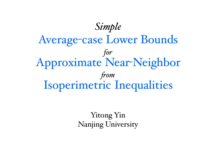
Simple Average - case Lower Bounds for Approximate Near - Neighbor fs om Isoperimetric Inequalities Yitong Yin Nanjing University
Nearest Neighbor Search ( NNS ) metric space ( X, dist) query x ∈ X database access y = ( y 1 , y 2 , . . . , y n ) ∈ X n data structure preprocessing x output : database point y i closest to the query point x applications : database, pattern matching, machine learning, ...
Near Neighbor Problem ( λ - NN ) metric space ( X, dist) query x ∈ X database access y = ( y 1 , y 2 , . . . , y n ) ∈ X n data structure radius λ preprocessing x λ λ - NN : answer “yes” if ∃ y i that is ≤ λ -close to x “no” if all y i are > λ -faraway from x
Approximate Near Neighbor ( ANN ) metric space ( X, dist) query x ∈ X database access y = ( y 1 , y 2 , . . . , y n ) ∈ X n data structure radius λ preprocessing x γλ λ approximation ratio γ ≥ 1 ( γ , λ ) - ANN : answer “yes” if ∃ y i that is ≤ λ -close to x “no” if all y i are > γλ -faraway from x arbitrary if otherwise
Approximate Near Neighbor ( ANN ) metric space ( X, dist) query x ∈ X database access y = ( y 1 , y 2 , . . . , y n ) ∈ X n data structure radius λ preprocessing x γλ λ approximation ratio γ ≥ 1 Hamming space X = { 0 , 1 } d dist( x, z ) = k x � z k 1 Hamming distance 100 log n < d < n o (1) Curse of dimensionality!
Cell-Probe Model data structure problem: query x ∈ X f ( x, y ) f : X × Y → Z database algorithm A : (decision tree) y ∈ Y t adaptive cell-probes table } w bits code T ( s cells (words) T : Y → Σ s where Σ = { 0 , 1 } w protocol: the pair ( A , T ) ( s , w , t ) -cell-probing scheme
Near - Neighbor Lower Bounds Hamming space X = { 0 , 1 } d database size: n d = Θ (log n ) time: t cell-probes; linear space: s = Θ ( n ) w = Θ ( d ) space: s cells, each of w bits Randomized Exact Approximate Near-Neighbor (ANN) Near-Neighbor Deterministic Randomized ( RENN ) ⇣ ⌘ ⇣ ⌘ t = Ω (1) d t = O(1) t = Ω (1) d t = Ω t = Ω log s log s [Miltersen et al. 1995] for s = poly( n ) [Borodin Ostrovsky Rabani 1999] [Barkol Rabani 2000] [Liu 2004] [Chakrabarti Regev 2004] ⇣ ⌘ ⇣ ⌘ d log n t = Ω ⇣ ⌘ ⇣ ⌘ t = Ω log n d t = Ω t = Ω log sw log log n ⇣ ⌘ ⇣ ⌘ log n n log sw log log n log n t = Ω t = Ω [P ă tra ş cu Thorup 2006] n log sw log log n [P ă tra ş cu Thorup 2006] n [Panigrahy Talwar Wieder ⇣ ⌘ d t = Ω (log n ) t = Ω log sw 2008, 2010] nd [Wang Y . 2014] • matches the highest known lower bounds for any data structure problems: Polynomial Evaluation [Larsen’12] , ball-inheritance (range reporting) [Grønlund, Larsen’16]
Why are data structure lower bounds so difficult? • (Observed by [Miltersen et al . 1995] ) An ω (log n ) cell-probe lower bound on polynomial space for any function in P would prove P ⊈ linear-time poly-size Boolean branching programs. (Solved in [Ajtai 1999] ) • (Observed by [Brody, Larsen 2012] ) Even non-adaptive data structures are circuits with arbitrary gates of depth 2: f ( x,y ) f : X × Y → Z f ( x’,y ) t fan-in table cells: s 1 arbitrary fan-in & -out data y y 1 y 2 y n -1 y n
Near - Neighbor Lower Bounds Hamming space X = { 0 , 1 } d database size: n time: t cell-probes; space: s cells, each of w bits Randomized Exact Approximate Near-Neighbor (ANN) Near-Neighbor Deterministic Randomized ( RENN ) ⇣ ⌘ ⇣ ⌘ d d t = Ω t = Ω log s log s [Miltersen et al. 1995] [Borodin Ostrovsky Rabani 1999] [Barkol Rabani 2000] [Liu 2004] ⇣ ⌘ d t = Ω ⇣ ⌘ d t = Ω log sw ⇣ ⌘ log n n log sw t = Ω [P ă tra ş cu Thorup 2006] n log sw [P ă tra ş cu Thorup 2006] n [Panigrahy Talwar Wieder ⇣ ⌘ d t = Ω log sw 2008, 2010] nd [Wang Y . 2014]
Average-Case Lower Bounds • Hard distribution: [Barkol Rabani 2000] [Liu 2004] [PTW’08 ’10] • database: y 1 ,..., y n ∈ {0,1} d i.i.d. uniform • query: uniform and independent x ∈ {0,1} d • Expected cell-probe complexity: • E ( x , y ) [ # of cell-probes to resolve query x on database y ] • “Curse of dimensionality” should hold on average. • In data-dependent LSH [Andoni Razenshteyn 2015] : a key step is to solve the problem on random input.
Average-Case Lower Bounds Hamming space X = { 0 , 1 } d database size: n time: t cell-probes; space: s cells, each of w bits Randomized Exact Approximate Near-Neighbor (ANN) Near-Neighbor Deterministic Randomized ( RENN ) ⇣ ⌘ ⇣ ⌘ d d t = Ω t = Ω log s log s [Miltersen et al. 1995] [Borodin Ostrovsky Rabani 1999] [Barkol Rabani 2000] [Liu 2004] ⇣ ⌘ d t = Ω ⇣ ⌘ d t = Ω log sw ⇣ ⌘ log n n log sw t = Ω [P ă tra ş cu Thorup 2006] n log sw [P ă tra ş cu Thorup 2006] n [Panigrahy Talwar Wieder ⇣ ⌘ d t = Ω log sw 2008, 2010] nd [Wang Y . 2014]
Average-Case Lower Bounds Hamming space X = { 0 , 1 } d database size: n time: t cell-probes; space: s cells, each of w bits Randomized Exact Approximate Near-Neighbor (ANN) Near-Neighbor Deterministic Randomized ( RENN ) ⇣ ⌘ ⇣ ⌘ d d t = Ω t = Ω log s log s [Miltersen et al. 1995] [Borodin Ostrovsky Rabani 1999] [Barkol Rabani 2000] [Liu 2004] our result: ⇣ ⌘ log n t = Ω log sw ⇣ ⌘ n d t = Ω [Panigrahy Talwar Wieder log sw nd 2008, 2010]
Metric Expansion [Panigrahy Talwar Wieder 2010] metric space ( X, dist) λ -neighborhood: ∀ x ∈ X, N λ ( x ) = { z ∈ X | dist( x , z ) ≤ λ } ∀ A ⊆ X, N λ ( A ) = { z ∈ X | ∃ x ∈ A s.t. dist( x , z ) ≤ λ } probability distribution μ over X • λ -neighborhoods are weakly independent under μ : ∀ x ∈ X, μ ( N λ ( x )) < 0.99/ n • λ -neighborhoods are ( Φ , Ψ ) -expanding under μ : ∀ A ⊆ X, μ ( A ) ≥ 1/ Φ ⇒ μ ( N λ ( A )) ≥ 1-1/ Ψ
Metric Expansion [Panigrahy Talwar Wieder 2010] probability distribution μ over X metric space ( X, dist) • λ -neighborhoods are ( Φ , Ψ ) -expanding under μ : ∀ A ⊆ X, μ ( A ) ≥ 1/ Φ ⇒ μ ( N λ ( A )) ≥ 1-1/ Ψ 1 / Φ 1 / Ψ vertex expansion, “blow-up” effect
Main Theorem: For ( γ , λ ) - ANN in metric space ( X, dist) where • γλ -neighborhoods are weakly independent under μ : μ ( N γλ ( x )) < 0.99/ n for ∀ x ∈ X • λ -neighborhoods are ( Φ , Ψ ) -expanding under μ : ∀ A ⊆ X that μ ( A ) ≥ 1/ Φ ⇒ μ ( N λ ( A )) ≥ 1-1/ Ψ ∀ deterministic algorithm that makes t cell-probes in expectation on a table of size s cells, each of w bits (assuming w +log s < n / log Φ ) , under the input distribution : database y =( y 1 , y 2 ,..., y n ) where y 1 , y 2 ,..., y n ∼ μ , i.i.d. query x ∼ μ , independently ! log Φ t = Ω sw log n log Ψ
Main Theorem: Hamming space X ={0,1} d , uniform distribution μ over X : For ( γ , λ ) - ANN in metric space ( X, dist) where choose γλ = d p 2 d ln(2 n ) 2 − • γλ -neighborhoods are weakly independent under μ : • γλ -neighborhoods are weakly independent under μ : μ ( N γλ ( x )) < 0.99/ n for ∀ x ∈ X μ ( N γλ ( x )) < 0.99/ n for ∀ x ∈ X • λ -neighborhoods are ( Φ , Ψ ) -expanding under μ : Harper’s Isoperimetric inequality : ∀ A ⊆ X that μ ( A ) ≥ 1/ Φ ⇒ μ ( N λ ( A )) ≥ 1-1/ Ψ ∀ A ⊆ X, μ ( A ) ≥ μ ( N r ( 0 )) ⇒ μ ( N λ ( A )) ≥ μ ( N r+ λ ( 0 )) ∀ deterministic algorithm that makes t cell-probes in expectation on a table of size s cells, each of w bits (assuming w +log s < n / log Φ ) , “Hamming balls have the smallest vertex-expansion.” under the input distribution : database y =( y 1 , y 2 ,..., y n ) where y 1 , y 2 ,..., y n ∼ μ , i.i.d. • λ -neighborhoods are (2 Θ ( d ) , 2 Θ ( d ) ) -expanding under μ : query x ∼ μ , independently ∀ A ⊆ X, μ ( A ) ≥ 2 - Θ ( d ) ⇒ μ ( N λ ( A )) ≥ 1-2 - Θ ( d ) ! log Φ 1 / Φ t = Ω ! ✓ ◆ d log Φ sw log t = Ω t = Ω n log Ψ log sw sw log 1 / Ψ n log Ψ nd
The Richness Lemma f ( x, y ) f : X × Y → { 0 , 1 } t log s y ∈ Y x ∈ X tw table ( s cells, each of w bits) cell-probing algorithm distributions μ over X, ν over Y α -dense: density of 1 s ≥ α under μ × ν monochromatic 1 -rectangle: A × B with A ⊆ X, B ⊆ Y s.t. ∀ ( x,y ) ∈ A × B, f ( x,y )=1 Richness lemma (Miltersen, Nisan, Safra, Wigderson, 1995) f has 1 -rectangle A × B with f is 0.01 -dense under μ × ν � μ ( A ) ≥ 2 -O( t log s ) n f has ( s , w , t ) - cell-probing scheme ν ( B ) ≥ 2 -O( t log s+ tw )
A New Richness Lemma distributions μ over X, ν over Y f : X × Y → { 0 , 1 } Richness lemma (Miltersen, Nisan, Safra, Wigderson, 1995) f has 1 -rectangle A × B with f is 0.01 -dense under μ × ν � μ ( A ) ≥ 2 -O( t log s ) n f has ( s , w , t ) - cell-probing scheme ν ( B ) ≥ 2 -O( t log s+ tw ) New Richness lemma f is 0.01 -dense under μ × ν � ∀ ∆ ∈ [320000 t , s ], f has 1 -rectangle A × B with f has average-case ( s , w , t )- cell-probing scheme μ ( A ) ≥ 2 -O( t log ( s / ∆ )) n under μ × ν ν ( B ) ≥ 2 -O( ∆ log ( s / ∆ ) + ∆ w ) when ∆ =O( t ) , it becomes the richness lemma (with slightly better bounds)
Recommend
More recommend
Explore More Topics
Stay informed with curated content and fresh updates.
