Automated Reasoning Induction Alan Bundy Automated Reasoning - PowerPoint PPT Presentation

Automated Reasoning Induction Alan Bundy Automated Reasoning Induction Lecture 14, page 1

A Summation Problem ● What is 1 + 2 + 3 + .... + 999 + 1000? ● Is there a formula for the general solution? ● Can we prove this? Automatically? Automated Reasoning Induction Lecture 14, page 2

A Summation Problem ● What is 1 + 2 + 3 + .... + 999 + 1000? ● Is there a formula for the general solution? ● Answer (due to Gauss): 1 + 2 + ... + n = ½ · n · ( n + 1) ● Can we prove this? Automatically? – Rewriting and model checking alone are not powerful enough, as there are an infinite number of cases. – We use the proof technique of induction (this lecture) and the automation heuristic rippling (next lectures). Automated Reasoning Induction Lecture 14, page 3

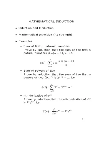
Mathematical Induction Gauss' theorem can be proved using a technique known as mathematical induction. The simplest form of mathematical induction proves that a statement holds for all natural numbers and consists of two steps: Base case: Show the statement holds for 0 Step case: Show that if the statement holds for any natural number n then it must hold for n +1 induction induction hypothesis (IH) conclusion (IC) Automated Reasoning Induction Lecture 14, page 4

Proving Gauss' Theorem To prove Gauss' theorem using this form of induction it is useful to start our summation at 0 (rather than 1): 0 + 1 + 2 + ... + n = ½ · n · ( n + 1) Proof : Base case: when n =0 we have 0 = ½ · 0 · 1 Step case: assume the formula holds for n ; then 0 + 1 + 2 + ... + n + ( n +1) = (0 + 1 + 2 + ... + n ) + ( n +1) by induction = ½ · n ·( n + 1) + 1·( n +1) hypothesis = (½· n + 1)·( n + 1) = (½)·( n +1)·( n +2) This shows that the formula holds for n +1 (QED). Automated Reasoning Induction Lecture 14, page 5

Types of Mathematical Induction ● So far, we have looked at weak induction: P  0  ∀ n:nat.P  n  P  s  n  ∀ n:nat.P  n  ● Complete induction is stronger: P  0  ∀ n:nat. ∀ k :nat.k ≤ n  P  k  P  s  n  ∀ n:nat.P  n  – Complete induction is used to prove the fundamental theorem of arithmetic, that every natural number is a product of primes. Automated Reasoning Induction Lecture 14, page 6

Recursive Functions Functions are often defined recursively (in terms of themselves). Induction is a natural way to prove many properties of such functions, e.g. even (0) = true even (s(0)) = false even (s(s(N))) = even (N) To prove even (2·n): Base case n =0 even (2 · 0) = even (0) = true Step case Assume induction hypothesis even (2· n ) We need to show even (2 · ( n +1)) even (2 · ( n +1)) = even (s(s(2 · n ))) (by rewriting) = even (2 · n ) (by definition) = true (by hypothesis) Automated Reasoning Induction Lecture 14, page 7

Recursive Datatypes: Lists ● Datatypes, such as lists, sets and trees, are also defined in a recursive manner. A list is defined as: – either the empty list (denoted by nil or [] ), or – an element combined with a list ● call the element h (head) and the list t (tail) ● the combination is written h #t (pronounced “ h cons t ”) ● Example: [ a , b , c ] = a # [ b , c ] = a # ( b # [ c ]) = a # ( b # ( c # []))) ● This is recursive: list is defined in terms of a list ● The function len can also be defined recursively: len (nil) = 0 len ( H#T )=s( len ( T )) Automated Reasoning Induction Lecture 14, page 8

Structural Induction ● To prove properties of recursive datatypes, we use a generalised type of induction called structural induction : To prove that a property holds for any instance of a recursively-defined structure, it is sufficient to prove: Base case: the property holds for the minimal structures in the definition Step case: if the property holds for the substructures of an arbitrary structure S then the property holds for S also. Automated Reasoning Induction Lecture 14, page 9

Well-Founded Orderings ● The induction argument uses the step case as follows: P(n) is true because P(n') is true, for some n ' < n ; and P(n') is true because P(n'') is true, for some n '' < n ' ; ... ● To be valid, this argument cannot go on forever – It requires an ordering; and – It must terminate (like our use of measures in lecture 8) – This is called a well-founded partial ordering ● Examples: – For the naturals, the usual ordering (less than) works – For lists, say L' < L whenever list L ' is the tail of list L . Under this ordering, nil is the unique minimal element Automated Reasoning Induction Lecture 14, page 10

Structural Induction (II) ● For lists, a structural induction proof that some property P holds for all lists consists of two parts. We must prove: P (1) P (nil) is true (2) if P ( t ) is true for any list t , then P ( h#t ) must be true for any h ● Our induction rule for lists can be written: P(nil), ∀ h:A. ∀ t :list(A). P(t) → P(h#t) ∀ l :list(A). P(l) Automated Reasoning Induction Lecture 14, page 11

Recursive Definitions (I) Append Two Lists: nil @ L = L ( H # T ) @ L = H # ( T @ L ) Convention that upper case letters are free List Membership: variables X mem nil = False X mem ( H # T ) = (if H=X then True else X mem T ) Butlast of a List: butlast nil = nil butlast ( H # T ) = (if T= nil then nil else H # butlast T) Automated Reasoning Induction Lecture 14, page 12

Recursive Definitions (II) Length of a List: len (nil) = 0 len ( H # T ) = s( len ( T )) Reverse a List: rev (nil) = nil rev ( H # T ) = rev ( T ) @ ( H # nil) (Quickly) Reverse a List: qrev (nil, L ) = L qrev ( H # T , L ) = qrev ( T , H # L ) Rotate a List: rot (0, L ) = L rot ( s( N ), nil) = nil rot ( s( N ), H # T ) = rot ( N , T @ ( H # nil)) Automated Reasoning Induction Lecture 14, page 13

Associativity of @ Convention that lower case letters are bound Conjecture: variables or constants ∀ k,l,m :list ( A ). k @ ( l @ m ) = ( k @ l ) @ m We need to choose a variable to induct on. If we use h#t - induction on k we get : Base Case: nil @ ( l @ m ) = (nil @ l ) @ m IH ( L and M are free variables ) Step Case: t @ (L @ M) = (t @ L) @ M ( h # t ) @ ( l @ m ) = (( h # t ) @ l ) @ m IC Automated Reasoning Induction Lecture 14, page 14

Proving the Base Case Rewrite rule: nil @ Y ⇒ Y (1) Equality Axiom (reflexivity): X=X no assumptions Proof: (the left of the sequent is empty) nil @ ( l @ m ) = (nil @ l ) @ m by (1) l @ m = (nil @ l ) @ m ⇔ by (1) l @ m = l @ m ⇔ true reflexivity ⇔ we use the convention that an not to be confused with ⇔ which was underlined term is being rewritten used for bi-directional rewriting to the purple term in the next line Automated Reasoning Induction Lecture 14, page 15

Proving the Step Case Rewrite rule: ( X # Y ) @ Z ⇒ X # ( Y @ Z ) (2) Proof: t @ (L @ M) = (t @ L) @ M ( h # t ) @ ( l @ m ) = (( h # t ) @ l ) @ m by (2) twice ⇔ h # ( t @ ( l @ m )) = ( h # ( t @ l )) @ m by (2) ⇔ h # ( t @ ( l @ m )) = h # (( t @ l ) @ m) replacement ⇔ h = h ∧ t @ ( l @ m ) = ( t @ l ) @ m by IH ⇔ h = h Since every step is reversible by reflexivity ⇔ true the induction conclusion is true given the induction hypothesis. Thus we have proven the step case. Automated Reasoning Induction Lecture 14, page 16

Fertilization ● In proving the step case we aim to make the IC resemble the IH – we want an instance of the IH to appear in the IC ● We then use the IH to prove the IC: Strong Fertilization ● Rewriting can get blocked before we reach an instance of the IH in the IC ● However, we may have part of the IH in the IC ● In this situation can use the IH as a rewrite rule: Weak Fertilization Automated Reasoning Induction Lecture 14, page 17

Theoretical Limitations of Inductive Inference Incompleteness: (Gödel) formal theories exclude some truths; examples found by Kirby & Paris. Undecidability of Halting Problem: (Turing) no algorithmic test for termination. Failure of Cut Elimination: (Kreisel) need to generalise and introduce lemmas. Automated Reasoning Induction Lecture 14, page 18

(Lack of) Cut Elimination Gentzen's Cut Rule: A ,   A ∇  ∇ lacks subformula property. Cut Elimination Theorem: Gentzen showed Cut Rule redundant in FOL. Kreisel showed necessary in inductive theories. Practical Consequences: Need to generalise conjectures. Need to introduce lemmas. Automated Reasoning Induction Lecture 14, page 19

Need for Intermediate Lemmas Conjecture: ∀ l :list( A ). rev ( rev ( l )) = l Rewrite rules: rev (nil) ⇒ nil (3) rev ( H # T ) ⇒ rev ( T ) @ ( H # nil) (4) Step Case: rev ( rev ( t )) = t rev ( rev ( h # t )) = h # t ⇔ rev ( rev ( t ) @ ( h # nil)) = h # t by (4) blocked Automated Reasoning Induction Lecture 14, page 20

Introducing an Intermediate Lemma Lemma Required: rev ( X @ Y ) = rev ( Y ) @ rev ( X ) (5) Cut Rule: introduces this Original:  rev ( rev ( l )) = l New:  , rev ( X @ Y ) = rev ( Y ) @ rev ( X ) rev ( rev ( l ))= l Justification:  rev ( X @ Y ) = rev ( Y ) @ rev ( X ) Heuristics are needed to speculate the lemma. Automated Reasoning Induction Lecture 14, page 21