Autocorrelation Estimates of Locally Stationary Time Series Srshti - PowerPoint PPT Presentation
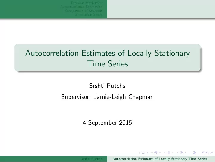
Problem Motivation Autocovariance Estimation Comparison of Methods Simulation Study Autocorrelation Estimates of Locally Stationary Time Series Srshti Putcha Supervisor: Jamie-Leigh Chapman 4 September 2015 Srshti Putcha Autocorrelation
Problem Motivation Autocovariance Estimation Comparison of Methods Simulation Study Autocorrelation Estimates of Locally Stationary Time Series Srshti Putcha Supervisor: Jamie-Leigh Chapman 4 September 2015 Srshti Putcha Autocorrelation Estimates of Locally Stationary Time Series
Problem Motivation Autocovariance Estimation Comparison of Methods Simulation Study Contents Problem Motivation 1 Problem Motivation Autocovariance Estimation 2 Rolling Windows Exponentially Weighted Windows Kernel Weighted Windows Comparison of Methods 3 Simulated Example ONS Economic Data Simulation Study 4 Simulation Study Conclusions Further Work Srshti Putcha Autocorrelation Estimates of Locally Stationary Time Series
Problem Motivation Autocovariance Estimation Problem Motivation Comparison of Methods Simulation Study Problem Motivation We often assume that time series are second-order stationary, with their statistical properties Quarterly Savings Data − Households & NPISH saving ratio remaining the same over time. 16 14 In reality, many time series are 12 % 10 not stationary and we shouldn’t 8 try to apply traditional methods. 6 4 This aim of this project 1970 1980 1990 2000 2010 Time was to explore and compare alternative methods of estimating Figure: Quarterly Savings Data time-varying autocovariance. UK (ONS). Srshti Putcha Autocorrelation Estimates of Locally Stationary Time Series
Problem Motivation Rolling Windows Autocovariance Estimation Exponentially Weighted Windows Comparison of Methods Kernel Weighted Windows Simulation Study Rolling Windows For a window length w , a time series can be segmented into T rolling windows. Then, the sample autocovariance can be Figure: Rolling windows for a time series of computed by: length T . Windowed Autocovariance At lag k and a window length w , w − k r k = 1 � ( x j − ¯ x )( x j + k − ¯ x ) . w j =1 Srshti Putcha Autocorrelation Estimates of Locally Stationary Time Series
Problem Motivation Rolling Windows Autocovariance Estimation Exponentially Weighted Windows Comparison of Methods Kernel Weighted Windows Simulation Study Exponentially Weighted Windows Using the same rolling window structure, we can instead weight the contributions of each observation within a window. Exponentially Weighted Autocovariance A value of β is selected such that 0 < β < 1. Then, w − k β j − 1 � q k = ( x j − ¯ x )( x j + k − ¯ x ) C k j =1 where C k = � w − k − 1 β i . i =0 Srshti Putcha Autocorrelation Estimates of Locally Stationary Time Series
Problem Motivation Rolling Windows Autocovariance Estimation Exponentially Weighted Windows Comparison of Methods Kernel Weighted Windows Simulation Study Kernel Weighted Windows For each individual window of the time series and lag k , the values ( x j − ¯ x )( x j + k − ¯ x ) from j = 1 , 2 , ..., ( w − k ) are weighted using a Gaussian Kernel. Gaussian Kernel The Kernel function is given by exp ( − z 2 1 K ( z ) = 2 ) . √ 2 π K ( z ) is nonnegative and integrates to 1. A weighted average is created and this is a localised estimate of the autocovariance of the time series at lag k . Srshti Putcha Autocorrelation Estimates of Locally Stationary Time Series
Problem Motivation Autocovariance Estimation Simulated Example Comparison of Methods ONS Economic Data Simulation Study Change in Variance This plot compares the various lag zero autocovariance estimates of a time series that exhibits a change in variance. Change in Variance (lag zero autocovariance) 15 Rolling Window Exponential Autocovariance 10 Kernel 5 0 0 200 400 600 800 1000 Windows Figure: Change in Variance Comparison (lag zero). Srshti Putcha Autocorrelation Estimates of Locally Stationary Time Series
Problem Motivation Autocovariance Estimation Simulated Example Comparison of Methods ONS Economic Data Simulation Study Quarterly Savings Data Differenced Quarterly Savings Data Comparison of Local Autocovariance Estimates (WL = 5) 4 15 Kernel Differenced Percentage Data Estimated Autocovariance Exponential (0.9) 2 Rolling Window 10 0 −2 5 −4 0 0 50 100 150 200 0 50 100 150 200 Time Window Figure: Left: Differenced data with changepoints, Right: Comparison of autocovariance methods. Srshti Putcha Autocorrelation Estimates of Locally Stationary Time Series
Problem Motivation Autocovariance Estimation Simulated Example Comparison of Methods ONS Economic Data Simulation Study Quarterly Savings Data Autocorrelation Estimates of Quarterly Savings Data (diff.) 1.0 0.5 Aucorrelation 0.0 −0.5 0 5 10 15 20 Lag Figure: Different autocorrelation estimates (t=55). Srshti Putcha Autocorrelation Estimates of Locally Stationary Time Series
Problem Motivation Simulation Study Autocovariance Estimation Conclusions Comparison of Methods Further Work Simulation Study Simulations The purpose of this simulation study was to compare the performance of the three methods. The study was conducted across seven different examples of simulated time series data, where changes were made to the second-order structure. Two important criteria were: Accuracy of the method (MSE). How robust the method was to window length. Srshti Putcha Autocorrelation Estimates of Locally Stationary Time Series
Problem Motivation Simulation Study Autocovariance Estimation Conclusions Comparison of Methods Further Work Simulation Study Simulation Example 1 A step change in variance was created halfway through the time series. The lag zero autocovariance estimates were compared to the simulated change in variance. Change in Variance − Simulation Average Change in Variance Comparison (Lag 0) 0.2 0.020 0.1 Average MSE 0.015 Rolling Window Data 0.0 Exponential (Beta=0.9) 0.010 Kernel −0.1 −0.2 0.005 0 200 400 600 800 1000 20 40 60 80 Time Window Length / Binwidth Figure: Left: Change in variance, Right: Comparison of methods (lag zero autocovariance). Srshti Putcha Autocorrelation Estimates of Locally Stationary Time Series
Problem Motivation Simulation Study Autocovariance Estimation Conclusions Comparison of Methods Further Work Simulation Study Simulation Example 1 Change in Variance − Exponential (Lag 0) 0.025 Beta = 0.8 Beta = 0.85 0.020 Beta = 0.9 Average MSE Beta = 0.95 0.015 0.010 0.005 20 40 60 80 Window Length Figure: Comparison across different beta values. Srshti Putcha Autocorrelation Estimates of Locally Stationary Time Series
Problem Motivation Simulation Study Autocovariance Estimation Conclusions Comparison of Methods Further Work Simulation Study Simulation Example 2 The simulated TVAR(1) model can be written as X t = α t X t − 1 + Z t , where Z t ∼ N (0 , 1) and α t evolves linearly over time (between − 0 . 5 and 0 . 5). The estimated lag one autocovariance was compared to a time-dependent theoretical equivalent γ t , α t γ t = . 1 − α 2 t Srshti Putcha Autocorrelation Estimates of Locally Stationary Time Series
Problem Motivation Simulation Study Autocovariance Estimation Conclusions Comparison of Methods Further Work Simulation Study Simulation Example 2 TVAR(1) − Simulation Average TVAR(1) − Comparison (Lag 1) 0.25 0.3 Rolling Window 0.20 0.2 Exponential (Beta=0.9) 0.1 Average MSE 0.15 Kernel Data 0.0 0.10 −0.1 0.05 −0.3 0.00 0 200 400 600 800 1000 20 40 60 80 Time Window Length Figure: Left: TVAR(1) simulation, Right: Comparison of methods (lag one autocovariance). Srshti Putcha Autocorrelation Estimates of Locally Stationary Time Series
Problem Motivation Simulation Study Autocovariance Estimation Conclusions Comparison of Methods Further Work Simulation Study Conclusions When statistical properties are constant for large sections of the time series, all methods perform in a similar manner. Srshti Putcha Autocorrelation Estimates of Locally Stationary Time Series
Problem Motivation Simulation Study Autocovariance Estimation Conclusions Comparison of Methods Further Work Simulation Study Conclusions When statistical properties are constant for large sections of the time series, all methods perform in a similar manner. The kernel weighted windows produce the most accurate estimates of nonstationary processes. Srshti Putcha Autocorrelation Estimates of Locally Stationary Time Series
Problem Motivation Simulation Study Autocovariance Estimation Conclusions Comparison of Methods Further Work Simulation Study Conclusions When statistical properties are constant for large sections of the time series, all methods perform in a similar manner. The kernel weighted windows produce the most accurate estimates of nonstationary processes. While dependent on β , the exponentially weighted windows were more robust to changes in window length, with flatter error curves. Srshti Putcha Autocorrelation Estimates of Locally Stationary Time Series
Recommend
More recommend
Explore More Topics
Stay informed with curated content and fresh updates.
