Atlantic Multidecadal Variability is Radiatively Forced. Mostly. - PowerPoint PPT Presentation

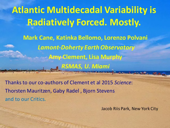
Atlantic Multidecadal Variability is Radiatively Forced. Mostly. Mark Cane, Katinka Bellomo, Lorenzo Polvani Lamont-Doherty Earth Observatory Amy Clement, Lisa Murphy RSMAS, U. Miami Thanks to our co-authors of Clement et al 2015 Science : Thorsten Mauritzen, Gaby Radel , Bjorn Stevens and to our Critics. Jacob Riis Park, New York City

Brooklyn NYC: Rockaway Jacob Riis Park and Marine Parkway Bridge Brooklyn

This talk is based on: Bellomo, K. N. Murphy, M. A. Cane, 2017, A. C. Clement, L.M. Polvani, L: Historical Forcings as Main • Drivers of the Atlantic Multidecadal Oscillation in the CESM Large Ensemble, Clim. Dyn.. DOI 10.1007/s00382-017-3834-3 Murphy , L.N., K. Bellomo, M. A. Cane, A. C. Clement, 2017: The Role of Historical Forcings in • Simulating the Observed Atlantic Multidecadal Oscillation, Geophys. Res. Lett. 44 (5), 2472-2480 10.1002/2016GL071337 Cane , M.A., A. C. Clement, L.N. Murphy, L.N., K. Bellomo, 2017: Low Pass Filtering, Heat Flux and • Atlantic Multidecadal Variability, J. Climate. 30 (18) 7529-7553 10.1175/JCLI-D-16-0810.1 Clement, A.C., M. A. Cane, L.N. Murphy, K. Bellomo, T. Mauritsen, B. Stevens, 2016: Response to • Comment on “The Atlantic Multidecadal Oscillation without a role for ocean circulation” Science 352 , (6293) 1527. [doi: 10.1126/science.aaf2575] Clement , A., K. Bellomo, L.N. Murphy, M.A. Cane, G. Rädel, B. Stevens, T. Mauritsen, 2015: The • Atlantic Multidecadal Oscillation Without a Role for Ocean Circulation. Science 350 , no. 6258, 320- 324.

OUTLINE Jacob Riis Park, New York City

NASST in Observations and CESM Large Ensembles NASST index 1920-2005 NASST index 1854-2005 (a)$NASST$index$(185422005);$LME (b)$NASST$index$(192022005);$LE Observed Observed LME mean LE mean NASST index = SST averaged over the North Atlantic (0-60N,80W-0) LME = Last Millennium Ensemble (10 members, CESM) LE = Large Ensemble (42 members, CESM) Light red = individual ensemble members Mean: the internal variations are averaged out; ≈ Forced Component only Bellomo et al. 2017

AMO: LE correlation with Observed 1920-2005 AMO index = NASST linearly detrended and LP filtered (20-year Lanczos filter) (d)$Corr.$Coeff.$with$obs 192022005 PDF over LE ensemble Pre-Industrial control (no historical forcing) LE minus mean (forcing removed) Random numbers All are detrended and LP filtered r of LE mean = .79 From Bellomo et al. 2017

AMO: LME correlation with Observed 1920-2005 AMO index = NASST linearly detrended and LP filtered (20-year Lanczos filter) (c)$Corr.$Coeff.$with$obs 185422005 PDF over LME ensemble Pre-Industrial control (no historical forcing) LME minus mean (forcing removed) Random numbers All are detrended and LP filtered r of LME mean = .72 From Bellomo et al. 2017

CMIP5 models without historical forcing do not produce agreement with observations Correlation with Observed AMO COLORS: External forcing (HIST) BLACK: No external forcing (Pre-industrial) Murphy et al. 2017

NASST Index Power Spectra LE: 1920-2005 LME: 1854-2005 LME all LE all Observed Observed LME de-meaned LE de-meaned LME mean LE mean NASST index = SST averaged over the North Atlantic (0-60N,80W-0) LME = Last Millennium Ensemble (10 members, CESM) LE = Large Ensemble (42 members, CESM) Light red = envelope of individual ensemble members Light blue = envelope of individual ensemble members, mean (forced part) removed From Bellomo et al. 2017

These correlations imply Bounds on INTERNAL/TOTAL variance in Observed AMO index MAX MIN . LME 1854-2005: 0.48 0.0 LE 1920-2005: 0.39 0.0 LME 1920-2005: 0.28 0.0 • Maximum is reached only if the model perfectly captures the forced response. (any takers?) • Minimum (0.0) means no internal variability at all. (Not credible.) A reasonable estimate for the observed is 20-40%; FORCED:INTERNAL ≈ 2:1. Model is ≈ 0.4 (too high) but model variance is too low What is the nature of the internal variability?

Coupled models (CMIP pre- industrial multimodel mean) reproduce this pattern! So do the same atmosphere models coupled to a slab ocean Clement et al. 2015

The fact that the coupled and slab results are so similar is a surprise, and creates a puzzle: How can the Atmosphere + (constant depth) Ocean Mixed Layer generate the same AMO patterns as a model with fully active ocean dynamics? • There is an ocean circulation and it surely transports heat and salt. • In the current prevailing paradigm, the ocean circulation (usually the AMOC) is considered essential for Atlantic Multidecadal Variability Lets look at the time/frequency behavior:

How do the temporal characteristics compare with and without interactive ocean dynamics? NB: All are PI runs; No External Forcing. All variability is Internal. NASST in CMIP3 slab models (red) NASST in coupled models and CMIP3 coupled models (blue) CMIP3 (blue) and CMIP5 (purple) • Slab and coupled, CMIP3,5 have the same variance • All look like red noise, without a multidecadal peak Clement et al 2015

No spectral peak in long model simulations (Ba et al. 2014)

The SST Equation may be written as dT/dt = -αT + q a + q o Q s v -αT is the turbulent flux (latent + sensible) damping q a are the other atmospheric fluxes – radiative, non-feedback turbulent fluxes Q s = -αT + q a is the total surface flux– the total heat exchange with the atmosphere q o is the ocean heat flux convergence + ocean mixed layer effects To enlighten us about Internal Variability in Pre-Industrial (no external forcing) GCMs, we go very simple: and take q a and q o to be white noise forcing . Cane et al. 2017

But are the ocean and atmosphere fluxes white? Wunsch, 1999; Stephenson et al 2001 say NAO is white. Spectra of Fluxes in the Coupled Model (CESM-CAM5) Qs = Surface Heat Flux Residual = dT/dt-Qs = Q_ocean Qs Residual dT/dt All quantities are averages over the AMO_mid region (60-20W, 40-55N) AMO_mid SST Cane et al. 2017

Comparison of AMO_mid from two Coupled Models (GFDL CM2.1, CCSM) with functions of the Filter Autocorrelation R(t) derived from white noise forced theory R(t)/R(0) r (T,T) R t (t)/[-R tt (0)R(0)] 1/2 r (dT/dt,T) -R tt (t)/[-R tt (0)] r (dT/dt, dT/dt) Cane et al. 2017

Correlation r (dT/dt,T) with varying (Butterworth) filter cutoff periods of 5, 10, 20, 30 years 10 20 5 30 NFM (noise forced model) White Noise Forced Model (NFM) 30 20 10 5 Periodic forcing T= sin(2 p t/60years) Periodic Forcing T = sin (2 (2 p /60 60 years) 10 20 5 30 10 20 5 30 Coupled Model (CESM) Coupled Model (CESM) (4 th order Butterworth filter) Cane et al. 2017

Low frequency forcing + noise dT/dt = -αT + q a + q o + c 2 sin( 2 p t/60years) q a , q o are white noise with variances ! 2 (q a )= a 2 ; ! 2 (q o )= b 2 Set a 2 = 0.85, b 2 = 0.15, c 2 = 0.1 Signal/Noise = c 2 /2 = 5% T(t) c 2 =0 r (dT/dt,T) With periodic c 2 = 0.1 Cane et al. 2017

Low frequency forcing + noise dT/dt = -αT + q a + q o + c 2 sin( 2 p t/60years) q a , q o are white noise with variances ! 2 (q a )= a 2 ; ! 2 (q o )= b 2 Set a 2 = 0.85, b 2 = 0.15, c 2 = 0.1 Signal/Noise = c 2 /2 = 5% T(t) c 2 =0 c 2 =0 r (dT/dt,T) With periodic c 2 = 0.1 -20 -15 -10 -5 0 5 10 15 20 Lag (years) Cane et al. 2017

But there is some evidence from decadal prediction work that ocean circulation matters in the Subpolar North Atlantic 2 − 5 yr lead 1 “Only correlation coefficients that exceed the 60 o N ‘no-skill’ statistical reference forecast at the 0.5 40 o N 90% confidence and exceed the NoInit* run 20 o N 0 0 o at 90% confidence are plotted.” − 0.5 20 o S 40 o S − 1 0 o 60 o E 120 o E 180 o W 120 o W 60 o W 0 o * Noinit = (small) HIST ensemble; 6 − 9 yr lead i.e. Externally Forced 1 60 o N 0.5 40 o N 20 o N 0 But perhaps not the buoyancy 0 o − 0.5 20 o S driven circulation -- the AMOC: 40 o S − 1 0 o 60 o E 120 o E 180 o W 120 o W 60 o W 0 o “…near-term prediction in this region may not rely on skillful AMOC prediction, only on adequate AMOC initialization—or more precisely, adequate initialization of temperature and salinity fields that support the correct geostrophic currents.” Piecuch et al. 2017 show it is wind-driven horizontal Karspeck et al. 2015 circulation (1994–2015) Figure 10

Conclusions

Th Thank You Jacob Riis Park, New York City

Rendered Figure 1 ��i�� �ere �� d��n���d Rendered Figure Figure� ��������� ��� �� ��1� 1��d� Rendered Figure 6 ��i�� �ere �� d��n���d Rendered Figure Figure� ��������� ��� �� ���6 6��d� SST vs. NAO Lead-Lag Correlations Models runs are PI Control + NAO_50yr Rendered Figure 6 ��i�� �ere �� d��n���d Rendered Figure Figure� ��������� ��� �� ���6 6��d� Observed Latitude La5tude Low Pass SST leads (b) Low Pass NAO leads SST lags SST leads Model A CM2.1_SLAB _Ctrl_NAO_50yr NAO leads SST leads Model B CM2.1 _Ctrl_NAO_50yr NAO leads SST leads Model C FLOR _Ctrl_NAO_50yr SST leads NAO leads SST leads SST lags Lag (years) Delworth et al. 2017 Figure 6 Lead-lag correla5ons between the SST response and the imposed NAO forcing Figures 1, 6