Asymptotic approximations for options with discrete sampling Sam - PowerPoint PPT Presentation
Asymptotic approximations for options with discrete sampling Sam Howison Mathematical Institute and Oxford-Man Institute for Quantitative Finance Oxford University 1 Preamble: Method of Multiple Scales (MMS) Asymptotic technique to resolve
Asymptotic approximations for options with discrete sampling Sam Howison Mathematical Institute and Oxford-Man Institute for Quantitative Finance Oxford University 1
Preamble: Method of Multiple Scales (MMS) Asymptotic technique to resolve slowly modulated fast oscilla- tions. Example: Oscillator � 2 ¨ x + x = 0 , 0 < � � 1 , has solution x ( t ) = e i t/� (rapid oscillation) and the substitution t = �τ gets us to x ′′ + x = 0 ( ′ = d / d τ ) . 2
If instead x + � 2 ˙ � 2 ¨ x + x = 0 , we also have small damping. In terms of τ , x ′′ + �x ′ + x = 0 . To approximate as � → 0, try x ( τ ; � ) ∼ x 0 ( τ ) + �x 1 ( τ ) + · · · . Then x ′′ x 0 = e i τ , 0 + x 0 = 0 , and x ′′ 1 + x 1 = − ie i τ . The solution has a term proportional to τ e i τ which grows un- boundedly in τ : secular term , not asymptotically correct if τ = O (1 /� ). 3
Remedy: use both τ and t as independent variables. Take � 2 d 2 x d t 2 + � 2 d x d t + x = 0 , and formally use τ and t with the chain rule d → ∂ ∂t + 1 ∂ d t − ∂τ . � 4
Then ∂ 2 x ∂ 2 x ∂ 2 x � � ∂t 2 + 2 ∂t∂τ + 1 � ∂x ∂t + 1 ∂x � � 2 + � 2 + x = 0 . � 2 ∂τ 2 � � ∂τ Expand x ( t, τ ; � ) ∼ x 0 ( t, τ ) + �x 1 ( t, τ ) + · · · and at leading order ∂ 2 x 0 ∂τ 2 + x 0 = 0 , so x 0 = A ( t )e i τ . Here A ( t ) is arbitrary . 5
Then at O ( � ), ∂ 2 x 0 ∂τ 2 + x 0 = − 2 ∂ 2 x 0 ∂t∂τ − ∂x 0 ∂τ − 2d A � � ie i τ . = d t − A ( t ) The RHS resonates with the LHS unless − 2d A d t − A ( t ) = 0 which gives the amplitude A ( t ) = e − t/ 2 . 6
Key features: • Introduce extra variable (embed problem) • New problem is degenerate ( A ( t ) arbitrary) at leading order • Resolve by solvability (orthogonality, Fredholm Alternative) at higher order. 7
Example: rapidly varying thermal conductivity. � ∂u ∂u ∂t = ∂ � x � � k ∂x � ∂x where k ( x/� ) is slowly varying – almost periodic on the scale � . Use x and X = x/� so that � 1 ∂X + ∂ ∂ � 1 ∂X + ∂u ∂u = ∂u � � �� k ( X ) ∂t . � ∂x � ∂x Expand u ( x, X, t ; � ) ∼ u 0 + �u 1 + � 2 u 2 and then at O ( � − 2 ) ∂ 2 u 0 ∂X 2 = 0 8
so that u 0 is a function of the slow variables x and t only. So also is u 1 but at O (1), we get + k ( X ) ∂ 2 u 0 ∂ k ( X ) ∂u 2 ∂x 2 = ∂u 0 � � ∂t . ∂X ∂X This is only consistent over one period of k if (integrate in X over the period and use periodicity of k ( X ) ∂u 2 /∂X ) � k � ∂ 2 u 0 ∂x 2 = ∂u 0 ∂t where � k � is the average of k .
Options in the Black-Scholes model The BS model is the standard description of normal (?!) financial markets. • Asset prices follow diffusions (SDEs driven by Wiener pro- cesses). • Options are contracts paying a given function P ( S T ), the payoff , of the asset price S T on a final date t = T . • Options are valued as expectations; thus... 9
• ... by Feynman-Kac, option prices satisfy a backward parabolic equation in S , t , with final data P ( S ): the BS PDE 2 σ 2 S 2 ∂ 2 V ∂V ∂S 2 + ( r − q ) S∂V ∂t + 1 ∂S − rV = 0 . Here r is the interest rate, q is the dividend rate and σ is the volatility.
A simple scaling and time-reversal t ′ = σ 2 ( T − t ) (so t ′ is dimensionless) turns 2 σ 2 S 2 ∂ 2 V ∂V ∂S 2 + ( r − q ) S∂V ∂t + 1 ∂S − rV = 0 . into 2 S 2 ∂ 2 V ∂V ∂S 2 + ( ρ − γ ) S∂V ρ = r γ = q ∂t ′ = 1 ∂S − ρV, σ 2 , σ 2 , with the payoff as initial data. 10
Discrete dividend payments When dividends are paid the asset price falls (in calendar time t ): S before = S after + dividend The model above has dividends paid continuously at rate q , asset price process d S t = ( r − q ) d t + σ d W t S t The corresponding scaled and forwardised BS PDE is 2 S 2 ∂ 2 V ∂V ∂S 2 + ( ρ − γ ) S∂V ρ = r γ = q ∂t ′ = 1 ∂S − ρV, σ 2 , σ 2 . 11
For discrete dividends, paying qS t − n δt at (equal) time intervals t n separated by δt , S t + n = (1 − q δt ) S t − n , or in scaled time T − t = σ 2 t ′ , � 2 = σ 2 δt . − = (1 − γ� 2 ) S t ′ S t ′ + , n n Between these dates, zero-dividend forwardised BS PDE holds: 2 S 2 ∂ 2 V ∂V ∂S 2 + ρS∂V ∂t ′ = 1 ∂S − ρV. 12
At dividend dates, option value is continuous for each realisa- + ) = V ( S t ′ − ) which is + , t ′ − , t ′ tion of S t , so V ( S t ′ n n n n + ) = V ((1 − γ� 2 ) S, t ′ − ) V ( S, t ′ n n for all 0 < S < ∞ . That is, the option values are shifted to the right across a dividend date (in backwards time). Value after before S 13
Discrete PDE + jump cond’s to cont’s PDE Multiple scale ansatz V ( S, t ′ , τ ) where t ′ = t ′ n + � 2 τ so discrete problem is 2 S 2 ∂ 2 V ∂V ∂t ′ + 1 ∂V ∂S 2 + ρS∂V ∂τ = 1 0 < τ < 1 ∂S − ρV, � 2 with V ( S, t ′ , 1 + ) = V ((1 − γ� 2 ) S, t ′ , 1 − ) and periodic in τ to eliminate secular terms, so V ( S, t ′ , 1 + ) = V ( S, t ′ , 0 + ) . 14
Expand V ∼ V 0 + � 2 V 1 + · · · and find V 0 = V 0 ( S, t ′ ) only; then ∂V 1 ∂τ = L V 0 , L = zero-div BS operator. So V 1 = τ L V 0 + F ( S, t ′ ) . Now expand jump cond’n to O ( � 2 ): V ( S, t ′ , 1 + ) = V ((1 − γ� 2 ) S, t ′ , 1 − ) ∼ V ( S, t ′ , 1 − ) − γ� 2 S∂V ∂S + · · · . Now the periodicity gives L V 0 = γS∂V 0 ∂S as required. 15
Asian options Asian options can be sampled discretely and depend on a running average n A t = 1 � S t i N 1 (can also do any function of S t ). Between the sample dates A t is constant and the option satisfies the BSPDE. At sampling dates the average is updated by i + 1 = A t − A t + N S t i . i 16
So the option value is updated by V ( S, t + i , A ) = V ( S, t − i , A − S t i /N ) (whatever A was before). Evidently the same machinery as for dividends can be used to derive the continuously sampled BS PDE 2 σ 2 S 2 ∂ 2 V ∂V ∂S 2 + rS∂V ∂S − rV + S∂V ∂t + 1 ∂A = 0 . This is particularly clear when the average is arithmetic and the payoff is affine in S and A , say max( S − A − K, 0): there is a similarity reduction V ( S, A, t ) = SW (( A − K ) /S, t ) where the average looks like a dividend payment in the equation for W . 17
American option with discrete dividend payments: Cox & Rubinstein p 250. 18
Recommend
More recommend
Explore More Topics
Stay informed with curated content and fresh updates.
