Assuming equal variances, can estimate using regression. E.g. for - PowerPoint PPT Presentation

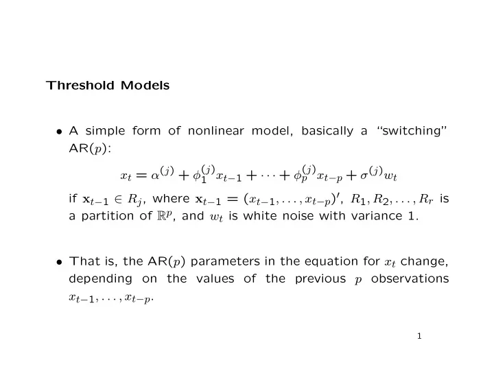
Threshold Models • A simple form of nonlinear model, basically a “switching” AR( p ): x t = α ( j ) + φ ( j ) 1 x t − 1 + · · · + φ ( j ) p x t − p + σ ( j ) w t if x t − 1 ∈ R j , where x t − 1 = ( x t − 1 , . . . , x t − p ) ′ , R 1 , R 2 , . . . , R r is a partition of R p , and w t is white noise with variance 1. • That is, the AR( p ) parameters in the equation for x t change, depending on the values of the previous p observations x t − 1 , . . . , x t − p . 1

• Assuming equal variances, can estimate using regression. E.g. for monthly pneumonia and influenza deaths: flu = ts(scan("flu.dat")); dflu = diff(flu); a = dflu; for (l in 1:6) a = cbind(a, lag(dflu, -l)); a = cbind(a, lag(dflu, -1) > 0.05); a = data.frame(a); names(a) = c("x", paste("x", 1:6, sep = ""), "delta"); summary(lm(x ~ delta + x1*delta + x2*delta + x3*delta + x4*delta + x5*delta + x6*delta, data = a)); flu.l = lm(x ~ -1 + delta + x1*delta + x2*delta + x3*delta + x4*delta, data = a); summary(flu.l); flu.r = residuals(flu.l); delta = a$delta[4 + 1:length(flu.r)]; lapply(split(flu.r, delta), sd); acf(flu.r); 2

• This is inefficient, and standard errors are invalid, if variances are unequal; here F = 1.93, df = (17, 110), P = .022. • We can also fit the model using two separate regressions: flu.lF = lm(x ~ x1 + x2 + x3 + x4, data = a, subset = (delta == 0)); summary(flu.lF); flu.lT = lm(x ~ x1 + x2 + x3 + x4, data = a, subset = (delta == 1)); summary(flu.lT); • Setting up a residual series: flu.r01 = flu.r; flu.r01[!delta] = residuals(flu.lF) / sd(residuals(flu.lF)); flu.r01[delta] = residuals(flu.lT) / sd(residuals(flu.lT)); acf(flu.r01); 3

Regression with Autocorrelated Errors • Regression model y t = β ′ z t + x t where x t has covariance matrix Γ . • Generalized least squares (GLS) estimates for known Γ : � − 1 Z ′ Γ − 1 y . � Z ′ Γ − 1 Z ˆ β = • For unknown Γ , plug in an estimate. 4

• If x t is a stationary time series, can fit using OLS, then either: – get estimated autocovariances ˆ γ ( h ) from the residuals, and plug in ˆ Γ ; – or use Cochrane-Orcutt method. • More generally, can use mixed model methods (SAS proc mixed ). 5

• Cochrane and Orcutt suggested: – fit using OLS to get initial estimate of β ; – fit AR( p ) to OLS residuals ( w t is white noise): φ ( B ) x t = w t ; – transform the regression to φ ( B ) y t = β ′ φ ( B ) z t + φ ( B ) x t = β ′ φ ( B ) z t + w t or u t = β ′ v t + w t . • Residuals are now white, so fit using OLS. 6

• SAS proc arima offers better solution: – Mortality and air pollution (Example 5.6): program and output. – Global temperature and cumulative CO 2 emissions: pro- gram and output. • In R, temperature (slightly different) and CO 2 : arima(globtemp, order = c(1, 0, 0), xreg = co2w); arima(globtemp, order = c(4, 0, 0), xreg = co2w); arima(globtemp, order = c(0, 0, 4), xreg = co2w); 7