Associative memories 9/25/2014 Memorized associations are - PowerPoint PPT Presentation
Associative memories 9/25/2014 Memorized associations are ubiquitous Stimulus Response Bill Memorized associations are ubiquitous Stimulus Response Key properties: Noise tolerance (generalization) Graceful saturation
Associative memories � 9/25/2014
Memorized associations are ubiquitous Stimulus Response “Bill”
Memorized associations are ubiquitous Stimulus Response Key properties: � • Noise tolerance (generalization) • Graceful saturation • High capacity “Bill”
First attempts: Holography van Heerden, 1963 Willshaw, Longuet-higgins, 1960s Z � r,s ( x ) = r ? s = r ( ⇣ ) r ( x − ⇣ ) d ⇣ Mathematically, this is the convolution-correlation scheme from class 4. Z s � φ r,s ( x ) = s ( τ ) φ r,s + ( τ + x ) d τ
Steinbuch, 1962 Matrix memories Willshaw et al., 1969 Input / Stimulus Before long, it was realized that better results could be obtained with a simpler, more neurally plausible framework. Let’s explore a simple Hebbian scheme. We have input and output lines, and we strength synapses when they’re on together. Output / Response
Storage
Storage
Storage
Storage
Storage What happens here depends on the specific choice of learning rule.
Storage S 3 S 2 S 1 Additive Hebb rule n X R i S T M = i i =1 What happens here R 1 depends on the R 2 specific choice of R 3 learning rule.
Storage S T M S 3 S 2 S 1 Additive Hebb rule n X R i S T M = i i =1 n X RS T M = i =1 What happens here R 1 depends on the R R 2 specific choice of R 3 learning rule.
Storage S T M S 2 Additive Hebb rule n X R i S T M = i i =1 n X RS T M = i =1
Storage S T M S 2 Additive Hebb rule n X R i S T M = i i =1 n X RS T M = i =1 ˆ ˆ R 2 R
Retrieval S T M S 1 Additive Hebb rule n X R i S T M = i i =1 n X RS T M = i =1
Retrieval S T M S 1 Additive Hebb rule n X R i S T M = i i =1 n X ˆ R i S T R j = i S j i =1 ˆ R 1 ˆ R
Retrieval S T M S 1 Additive Hebb rule n X R i S T M = i i =1 n X ˆ R i S T R j = i S j i =1 n X ˆ R i S T i S j + R j || S j || 2 R j = ˆ R 1 ˆ R i 6 = j
Retrieval S T M S 1 Additive Hebb rule n X R i S T M = i i =1 n X ˆ R i S T R j = i S j i =1 0 1 n X ˆ R i S T i S j + R j || S j || 2 R j = ˆ R 1 ˆ R i 6 = j If the S k are orthonormal , then retrieval is exact.
Another perspective Recall the the optimal memory matrix is M ? = RS † If the columns of S are linearly independent, then X † = ( X T X ) − 1 X T , giving M ? = R ( S T S ) − 1 S T . So if the columns of S (the S i ) are orthonormal, M ? = RS T , which is exactly what we got for the simple Hebb rule.
Capacity How much information can a matrix memory store? Model: P patterns of size N 1. | S | = | R | = N × P 2. Each input pattern (column of S ) has m S nonzeros, and each output pattern (column of R ) has m R nonzeros. 3. Binary Hebb rule: M = max( RS T , 1 ) (Each entry is clipped at one.) 4. Threshold recall: ⇢ 1 [ M S j ] k > τ ˆ R jk = 0 else
Capacity How much information can a matrix memory store? Model: P patterns of size N 1. | S | = | R | = N × P 2. Each input pattern (column of S ) has m S nonzeros, and each output pattern (column of R ) has m R nonzeros. 3. Binary Hebb rule: M = max( RS T , 1 ) � (Each entry is clipped at one.) Parameters we can pick 4. Threshold recall: ⇢ 1 [ M S j ] k > τ ˆ R jk = 0 else
Capacity S T M To choose the threshold τ , note that in the absence of noise, a column of M has exactly m S ones. So in order to recover all the ones in R , we better set τ = m S . ˆ ˆ R 2 R
Capacity Sparsity parameters The chance of given weight in M remaining zero throughout the learning process is (1 − m S m R − P mS mR ) P ≈ e = (1 − q ) N 2 N 2 The probability of a spurious one in ˆ R is the probability of exceeding τ purely by chance. This is Nq m S . So the highest value for m S we can choose before make the first error is: m S = − log N Nq m S = 1 ⇒ log q
Capacity From previous slide Sparsity parameters − P mS mR m S = − log N = (1 − q ) N 2 e log q
Capacity Sparsity parameters This is quite good! = log(2) m S m R − P mS mR (1 − q ) = e N 2 ⇒ N 2 N 2
Kanerva, 1988 Memory space The decision to represent memory items as sparse, high- dimensional vectors has some interesting consequences. High-dimensional spaces are counterintuitive. In 1000 dimensions, 0.001 of all patterns are within 451 bits of a given point, and all but 0.001 are within 549 bits. � Points tend to be orthogonal - most point-pairs are “noise-like.”
Kanerva, 1988 Memory space The decision to represent memory items as sparse, high- dimensional vectors has some interesting consequences. High-dimensional spaces are counterintuitive. Linking concepts Almost all pairs of points are far apart, but there are multiple“linking” points that are close to both. �
Kanerva, 1988 Memory space The decision to represent memory items as sparse, high- dimensional vectors has some interesting consequences. High-dimensional spaces are counterintuitive. Linking concepts Almost all pairs of points are far apart, but there are multiple“linking” points that are close to both. �
Matrix memories in the brain: Marr, 1967 Albus, 1971 Marr’s model of the cerebellum Short, live experiment
Matrix memories in the brain: Marr’s model of the cerebellum The cerebellum produces smooth , coordinated motor movements. (And may be involved in cognition as well). 24-year old Chinese woman without a cerebellum
Learn associations straight Purkinje Axons from context to actions, so Motor Output you don’t have to “think” before doing. Mossy Fiber Contextual Input
Learn associations straight Purkinje Axons from context to actions, so Motor Output you don’t have to “think” before doing. Mossy Fiber Contextual Input
Learn associations straight Purkinje Axons from context to actions, so Motor Output you don’t have to “think” before doing. Mossy Fiber Contextual Input
But how does training work? Purkinje Axons How do the right patterns Motor Output “appear” on the output (Purkinje) lines? Mossy Fiber Contextual Input Climbing Fibers Motor Teaching Input The rest of the brain
Purkinje Axons There’s a remarkable 1-1 correspondence Motor Output between climbing fibers and Purkinje axons. Moreover, each climbing fiber wraps around and around it’s Purkinje axon, making hundreds of synapses; a single AP can make a Purkinje spike. Mossy Fiber Contextual Input Climbing Fibers Motor Teaching Input The rest of the brain
We said that sparsity was a Purkinje Axons key property. How is that Motor Output manifested here? Mossy Fiber Contextual Input Climbing Fibers Motor Teaching Input The rest of the brain
Purkinje Axons Motor Output Granule Cells Sparsification Mossy Fiber Contextual Input Climbing Fibers Motor Teaching Input
Purkinje Axons Motor Output Granule Cells Sparsification Mossy Fiber Contextual Input Climbing Fibers Motor Teaching Input
Purkinje Axons Motor Output Granule Cells Sparsification Mossy Fiber Contextual Input Climbing Fibers Motor Teaching Input
Purkinje Axons Motor Output Granule Cells Sparsification There are 50 billion granule cells - 3/4 of the brain’s neurons.They’re tiny. � The idea here is that they “blow up” the mossy fiber input into a larger space in Mossy Fiber which the signal can be sparser. Contextual Input � Granule cells code for sets of mossy fibers Climbing Fibers Motor Teaching Input ( codons ), hypothesized to be primitive input features.
Storing structured information We’ve discussed how to store S-R pairs, but human cognition goes way beyond this. Relations � • The kettle is on the table. • The kettle is to the right of the mug.
Storing structured information As before, “concepts” are activation vectors. Kettle Jar
Storing structured information As before, “concepts” are activation vectors. How to represent this? Green(Jar) & Gray(Kett le) Kettle Jar
Storing structured information As before, “concepts” are activation vectors. How to represent this? Green(Jar) & Gray(Kett le) Kettle Jar Green Gray
Storing structured information As before, “concepts” are activation vectors. How to represent this? Now what? Maybe we should just have Green(Jar) & Gray(Kett le) all of these patterns fire at once? � But then how do we know we don’t Kettle Jar Green Gray have Gray(Jar) & Green(Kettle) ? Or, worse, Jar(Kettle) & Green & Gray?
Storing structured information As before, “concepts” are activation vectors. How to represent this? Now what? Maybe we should just have Green(Jar) & Gray(Kett le) all of these patterns fire at once? � But then how do we know we don’t Kettle Jar Green Gray have Gray(Jar) & Green(Kettle) ? Or, worse, Jar(Kettle) & Green & Gray? We need a way to bind predicates to arguments.
Storing structured information As before, “concepts” are activation vectors. How to represent this? We need a way to bind Green(Jar) & Gray(Kett le) predicates to arguments. Green Gray Kettle Jar Binding operator ⊗ ⊕ ⊗ Conjunction operator
Recommend
More recommend
Explore More Topics
Stay informed with curated content and fresh updates.
