Assessing the PH Assumption So far, weve been considering the - PowerPoint PPT Presentation

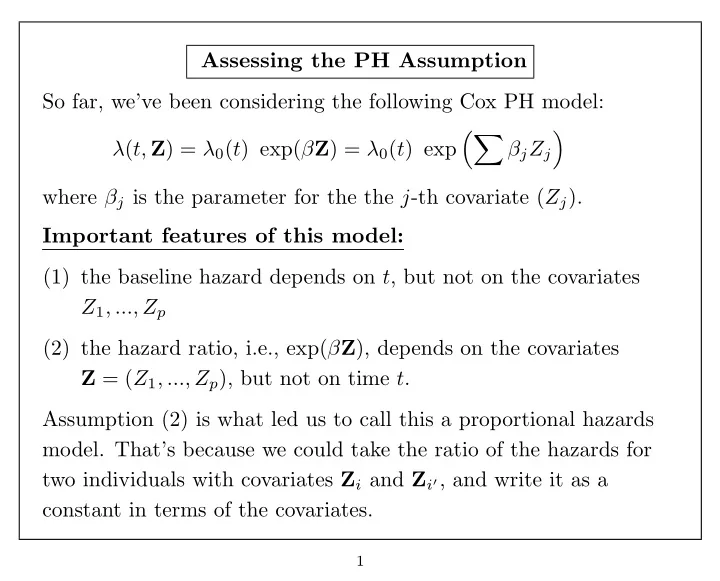
Assessing the PH Assumption So far, we’ve been considering the following Cox PH model: �� � λ ( t, Z ) = λ 0 ( t ) exp( β Z ) = λ 0 ( t ) exp β j Z j where β j is the parameter for the the j -th covariate ( Z j ). Important features of this model: (1) the baseline hazard depends on t , but not on the covariates Z 1 , ..., Z p (2) the hazard ratio, i.e., exp( β Z ), depends on the covariates Z = ( Z 1 , ..., Z p ), but not on time t . Assumption (2) is what led us to call this a proportional hazards model. That’s because we could take the ratio of the hazards for two individuals with covariates Z i and Z i ′ , and write it as a constant in terms of the covariates. 1

Proportional Hazards Assumption Hazard Ratio: λ ( t, Z i ) λ 0 ( t ) exp( β Z i ) = λ ( t, Z i ′ ) λ 0 ( t ) exp( β Z i ′ ) exp( β Z i ) = exp( β Z i ′ ) = exp[ β ( Z i − Z i ′ )] � = exp[ β j ( Z ij − Z i ′ j )] = θ In the last formula, Z ij is the value of the j -th covariate for the i -th individual. For example, Z 42 might be the value of gender (0 or 1) for the the 4-th person. 2

We can also write the hazard for the i -th person as a constant times the hazard for the i ′ -th person: λ ( t, Z i ) = θ λ ( t, Z i ′ ) Thus, the HR between two types of individuals is constant (i.e., = θ ) over time. These are mathematical ways of stating the proportional hazards assumption. 3

There are several options for checking the assumption of proportional hazards: I. Graphical (a) Plots of survival estimates for two subgroups (b) Plots of log[ − log( ˆ S )] vs log( t ) for two subgroups (c) Plots of weighted Schoenfeld residuals vs time (d) Plots of observed survival probabilities versus expected under PH model (see Kleinbaum, ch.4) II. Use of goodness of fit tests - we can construct a goodness-of-fit test based on comparing the observed survival probability (from sts list ) with the expected (from stcox ) under the assumption of proportional hazards - see Kleinbaum ch.4 III. Including interaction terms between a covariate and t (time-dependent covariates) 4

How do we interpret the above? Kleinbaum (and other texts) suggest a strategy of assuming that PH holds unless there is very strong evidence to counter this assumption: • estimated survival curves are fairly separated, then cross • estimated log cumulative hazard curves cross, or look very unparallel over time • weighted Schoenfeld residuals clearly increase or decrease over time (you could fit a OLS regression line and see if the slope is significant) • test for time × covariate interaction term is significant (this relates to time-dependent covariates) 5

If PH doesn’t exactly hold for a particular covariate but we fit the PH model anyway, then what we are getting is sort of an average HR, averaged over the event times. In most cases, this is not such a bad estimate. Allison claims that too much emphasis is put on testing the PH assumption, and not enough to other important aspects of the model. 6

Implications of proportional hazards Consider a PH model with a single covariate, Z: λ ( t ; Z ) = λ 0 ( t ) e βZ What does this imply for the relation between the survivorship functions at various values of Z? Under PH, log[ − log[ S ( t ; Z )]] = log[ − log[ S 0 ( t )]] + βZ 7

In general, we have the following relationship: � t Λ i ( t ) = λ i ( u ) du 0 � t = λ 0 ( u ) exp( β Z i ) du 0 � t = exp( β Z i ) λ 0 ( u ) du 0 = exp( β Z i ) Λ 0 ( t ) This means that the ratio of the cumulative hazards is the same as the ratio of hazard rates: Λ i ( t ) = exp( β Z i ) = exp( β 1 Z 1 i + · · · + β p Z pi ) Λ 0 ( t ) 8

Using the above relationship, we can show that: � Λ i ( t ) � β Z i = log Λ 0 ( t ) = log Λ i ( t ) − log Λ 0 ( t ) = log[ − log S i ( t )] − log[ − log S 0 ( t )] so log[ − log S i ( t )] = log[ − log S 0 ( t )] + β Z i Thus, to assess if the hazards are actually proportional to each other over time • calculate Kaplan Meier Curves for various levels of Z • compute log[ − log( ˆ S ( t ; Z ))] (i.e., log cumulative hazard) • plot vs log-time to see if they are parallel (lines or curves) Note: If Z is continuous, break into categories. 9

Question: Why not just compare the underlying hazard rates to see if they are proportional? Here’s two simulated examples with hazards which are truly proportional between the two groups: Weibull-type hazard: U-shaped hazard: Plots of hazard function vs time Simulated data with HR=2 for men vs women Plots of hazard function vs time Simulated data with HR=2 for men vs women HAZARD 0.010 HAZARD 0.010 0.008 0.008 0.006 0.006 0.004 0.004 0.002 0.002 0.000 0.000 0 100 200 300 400 500 600 700 800 900 1000 1100 0 100 200 300 400 500 600 700 800 900 1000 1100 Length of Stay (days) Length of Stay (days) Gender Women Men Gender Women Men 10

Reason 1: It’s hard to eyeball these figures and see that the hazard rates are proportional - it would be easier to look for a constant shift between lines. Reason 2: Estimated hazard rates tend to be more unstable than the cumulative hazard rate 11

Consider the nursing home example (where we think PH is reasonable). If we group the data into intervals and calculate the hazard rate using actuarial method, we get these plots: 200 day intervals: 100 day intervals: Plots of hazard function vs time Plots of hazard function vs time 0.006 0.009 0.008 0.005 0.007 0.004 0.006 0.005 0.003 0.004 0.002 0.003 0.002 0.001 0.001 0.000 0.000 0 100 200 300 400 500 600 700 800 900 1000 0 100 200 300 400 500 600 700 800 900 1000 Length of Stay (days) Length of Stay (days) Gender Women Men Gender Women Men 12

50 day intervals: 25 day intervals: Plots of hazard function vs time Plots of hazard function vs time 0.012 0.014 0.012 0.010 0.010 0.008 0.008 0.006 0.006 0.004 0.004 0.002 0.002 0.000 0.000 0 100 200 300 400 500 600 700 800 900 1000 1100 0 100 200 300 400 500 600 700 800 900 1000 1100 Length of Stay (days) Length of Stay (days) Gender Women Men Gender Women Men 13

In contrast, the log cumulative hazard plots are easier to interpret and tend to give more stable estimates Stata has two commands which can be used to graphically assess the proportional hazards assumption: • stphplot: plots − log[ − log( − ( S ( t ))] curves for each category of a nominal or ordinal independent variable versus log(time). Optionally, these estimates can be adjusted for other covariates. • stcoxkm: plots Kaplan-Meier observed survival curves and compares them to the Cox predicted curves for the same variable. (No need to run stcox prior to this command, it will be done automatically) For either command, you must have stset your data first. You must specify by() with stcoxkm and you must specify either by() or strata() with stphplot . 14

Ex: Nursing Home - gender . use nurshome . stset los fail . label define sexlab 1 "Males" 0 "Females" . label val gender sexlab . stphplot, by(gender) noneg title(Evaluation of PH Assumption) Evaluation of the PH assumption 2 ln[ln(Survival Probability)] 0 2 4 6 0 2 4 6 8 ln(analysis time) gender = Females gender = Males We use the option noneg to plot the log[ − log( S ( t ))] cuves rather than the − log[ − log( S ( t ))] curves that are the STATA default. 15

Ex: Nursing Home - marital status . label define marlab 1 "Married" 0 "Not married" . label val married marlab . stphplot, by(married) noneg title(Evaluation of PH Assumption) Evaluation of the PH assumption 2 ln[ln(Survival Probability)] 0 2 4 0 2 4 6 8 ln(analysis time) married = Not married married = Married This is equivalent to comparing plots of the log cumulative hazard, log(ˆ Λ( t )), between the covariate levels, since � t Λ( t ) = λ ( u ; Z ) du = − log[ S ( t )] 0 16

Assessing proportionality with several covariates If there is enough data and you only have a couple of covariates, create a new covariate that takes a different value for every combination of covariate values. Example: Health status and gender for nursing home . use nurshome . gen hlthsex=1 if gender==0 & health==2 . replace hlthsex=2 if gender==1 & health==2 . replace hlthsex=3 if gender==0 & health==5 . replace hlthsex=4 if gender==1 & health==5 . label define hsfmt 1 "Healthier Women" 2 "Healthier Men" > 3 "Sicker Women" 4 "Sicker Men" . label val hlthsex hsfmt 17

Log[-log(survival)] Plots for Health status*gender . stphplot, by(hlthsex) noneg 1 0 ln[ln(Survival Probability)] 1 2 3 4 0 2 4 6 8 ln(analysis time) hlthsex = Healthier Women hlthsex = Healthier Men hlthsex = Sicker Women hlthsex = Sicker Men If there are too many covariates (or not enough data) for this, then there is a way to test proportionality for each variable, one at a time, using the stratification option. 18

What if proportional hazards fails? • do a stratified analysis • include a time-varying covariate to allow changing hazard ratios over time • include interactions with time The second two options relate to time-dependent covariates, which is getting beyond the scope of this course. We will focus on the first alternative, and then the second two options will be briefly described. 19