Applying Cost Curves to Marine Cargo Container Inspection DIMACS / - PowerPoint PPT Presentation
Applying Cost Curves to Marine Cargo Container Inspection DIMACS / DyDAn / LPS Workshop on Port Security, Safety, Inspection, Risk Analysis and Modeling Rutgers University November 18 th , 2008 Richard Hoshino Laboratory and Scientific
Applying Cost Curves to Marine Cargo Container Inspection DIMACS / DyDAn / LPS Workshop on Port Security, Safety, Inspection, Risk Analysis and Modeling Rutgers University November 18 th , 2008 Richard Hoshino Laboratory and Scientific Services Directorate Canada Border Services Agency
Context • Each year in Canada, approximately 20,000 marine containers are referred for a full examination. • Some of these containers have been fumigated with chemical compounds to kill invasive alien species. • If these marine containers are not ventilated properly, fumigants may pose a risk to the health and safety of border service officers. 1
Flowchart of Current Process Test Positive Negative Start Exam Ventilate Test Positive Negative Exam 2
A Simple Yet Powerful Insight • We can create a mathematical model that predicts whether a container has been fumigated. • For containers predicted to have been fumigated, we ventilate prior to testing. • Deploying a reliable binary classifier would reduce the overall costs of inspection, creating a more efficient and effective port. 3
Flowchart of Proposed Process Test Predict Non-Fumigated Positive Negative Model Predict Fumigated Exam Ventilate Start Test Positive Negative Exam 4 Predict Non-Fumigated : Test first Predict Fumigated : Ventilate first
Misclassification Cost • The misclassification cost of the Status Quo is M 1 = #P × $C − • The misclassification cost of the Binary Classifier is M 2 = #FN × $C − + #FP × $C + = ( FNR × #P) × $C − + ( FPR × #N) × $C + = (1 − TPR ) × #P × $C − + FPR × #N × $C + • Given a predictive model, its optimal binary classifier is the classifier that minimizes the misclassification cost M 2 . 5
The Improvement Curve • We introduce the improvement curve , inspired by the theory of cost curves (Drummond & Holte, 2000). • Improvement curves measure a model’s performance – Over all possible class distributions ( #P vs. #N ) – Over all possible misclassification costs ( $C − and $C + ) • Define the improvement to be I = (M 1 − M 2 ) ÷ M 1 . 0% IMPROVEMENT % 100% Same as Status Quo This Model’s Perfect Model 6 FPR = 0, FNR = 1 Best Classifier FPR = 0, FNR = 0
Definition of x -axis and y -axis • The x -axis of the improvement curve is the following expression, denoted as probability times cost : x = PC(+) = (#P × $C − ) ÷ (#P × $C − + #N × $C + ) . • The y -axis is the improvement , the percentage reduction in misclassification cost by replacing the status quo with the model’s optimal classifier: y = I(x) = (M 1 − M 2 ) ÷ M 1 = TPR − [ FPR × (#N × $C + ) ÷ (#P × $C − ) ] . 7 It is straightforward to show that 0 ≤ x ≤ 1 and 0 ≤ y ≤ 1.
Illustrating the Theory • We built a simple predictive model based on a 4,200 container data set. The model’s four features are: – Origin Country – Canadian Port of Arrival – HS section (e.g. Section 5 = Mineral Products) – HS chapter (e.g. Chapter 26 = Ores, Slag, Ash) • The model consists of 2 4 =16 disjoint classes. • The data was split 70/30 for Training/Testing. 8
ROC Curve of Model ROC AUC Training = 0.75 Testing = 0.74 9
Improvement Curve of Model Training = Red Testing = Blue 10
Improvement Curve Interpretation • Suppose #N ÷ #P = 6 and $C − ÷ $C + = 4 . Then, x = PC(+) = (#P × $C − ) ÷ (#P × $C − + #N × $C + ) = 0.4 . • From the improvement curve, we have y = 28% (Reading from the Testing Set). • This simple 4-feature model would have reduced our misclassification cost by 28%. 0% 28% 100% Same as Status Quo This Model’s Best Classifier Perfect Model 11 FPR = 0, FNR = 1 FPR=20.3%, TPR=62.5% FPR = 0, FNR = 0
Conclusion • The Improvement Curve does the following: – Addresses the limitations of ROC curves and the ROC AUC. – Measures performance over all possible values of PC(+). – Determines a simple condition for when the status quo should be retained. – Compares the optimal classifiers of two predictive models. • The Improvement Curve is an evaluation metric that – Is extremely accessible to a non-specialist. – Has numerous applications to operations research beyond marine container inspection. 12
Recommend
More recommend
Explore More Topics
Stay informed with curated content and fresh updates.
