Applications of Diffusion Models in Telecommunications Nigel Meade - PowerPoint PPT Presentation
Applications of Diffusion Models in Telecommunications Nigel Meade 2 Introduction Recent examples of diffusion in telecomms Definition of diffusion model Survey of telecomms applications Extrapolation Use of explanatory
Applications of Diffusion Models in Telecommunications Nigel Meade
2 Introduction •Recent examples of diffusion in telecomms •Definition of diffusion model •Survey of telecomms applications •Extrapolation •Use of explanatory variables •Inter-market models •Multi - national •Multi - generation •Multi - technology •Strengths •Weaknesses
3 Recent examples of diffusion in telecomms - 1 Financial Times 20/9/2004
4 Recent examples of diffusion in telecomms – 1a Potential penetration of 20 million households Rapid Growth Gradual growth Growth quickly evapoarates Financial Times 20/9/2004
5 Recent examples of diffusion in telecomms - 2 Financial Times 22/9/2004
6 Recent examples of diffusion in telecomms – 2a No obvious limit to potential penetration Rapid Exponential Growth Gradual linear growth Growth to a saturation level Financial Times 22/9/2004
7 Recent examples of diffusion in telecomms - 3 Financial Times 21/9/2004
8 Recent examples of diffusion in telecomms - 4 3G starts to attract 2G customers Forbes 20/9/2004
9 Definition of Diffusion models • A new technology diffuses Saturation level into a population Early Adopters Early Majority Adoption per Period Cumulative Adoption Late Majority Laggards 0 10 20 30 40 50 60 70 80 90 100 Time
10 Example – UK Colour TV UK Adoption of Colour TV Early Adopter s Early Majority Adoption per Period Cumulative Adoption Laggards Late Majority 0 5 10 15 20 25 30 35 40 45 Time
11 Forecasting Issues of Interest • What will the rate of adoption be at a particular time? • How many potential adopters are there in total? • When will peak demand occur? • How high is peak demand?
12 Problems in Forecasting • Identify the appropriate model • Estimate its parameters • Predict future adoption – (with a prediction interval). • Model identification is crucial – the literature reveals 29 possible models – there is no best single model
13 A selection of diffusion models Gompertz Logistic Log Reciprocal 1 1 1 0.8 0.8 0.8 Penetration (Xt) Penetration (Xt) Penetration (Xt) 0.6 0.6 0.6 0.4 0.4 0.4 0.2 0.2 0.2 0 0 0 0 10 20 30 40 50 0 10 20 30 40 50 0 10 20 30 40 50 Time (t) Time (t) Time (t) Cumulative Lognormal Extended Logistic (A) Weibull 1 1 1 0.8 0.8 0.8 Penetration (Xt) Penetration (Xt) Penetration (Xt) 0.6 0.6 0.6 0.4 0.4 0.4 0.2 0.2 0.2 0 0 0 0 10 20 30 40 50 0 10 20 30 40 50 0 10 20 30 40 50 Time (t) Time (t) Time (t)
14 Model identification • Meade & Islam (Management Science 1998) • The best fitting model is not necessarily the best forecasting model • They propose combining criteria based on: – Model fit (measured by R 2 – Model stability (looks at one step ahead forecasts) • These criteria suggest a subset of models which are used to produce a combined forecast
15 Forecasting Cable Television Penetration in US 0.6 0.6 0.6 Forecast Forecast Forecast Region Region Region 0.5 0.5 0.5 CATV Penetration in US CATV Penetration in US CATV Penetration in US Forecast of Forecast of Forecast of Estimation Region Estimation Region Estimation Region 0.4 0.4 0.4 Best fitting model Best fitting model Best fitting model Combined Combined 0.3 0.3 0.3 Forecast Forecast 0.2 0.2 0.2 0.1 0.1 0.1 0 0 0 0 5 10 15 20 25 30 35 0 0 5 5 10 10 15 15 20 20 25 25 30 30 35 35 Time Time Time
16 Applications in Telecomms Variable Author Model Chaddha & Logistic Chitgokepar (1971) Hyett & McKenzie Logistic (1975) Fixed line telephone Bewley & Fiebig Flexible logistic penetration (1988) Lee et al (1992) Non-linear growth Meade & Islam Comparison of 14 (1995) models Business Meade & Islam Growth + Telephones (1996) econometric
17 Modelling approaches • Extrapolate from available data 12 UK Business Telephones (Mil) 10 8 Fixed Saturation Level 6 4 Actual Telephones 2 0 1955 1960 1965 1970 1975 1980 1985 1990 1995 Date
18 Modelling approaches • Dynamic saturation level by relation to environmental variables 12 Implied Saturation Level (local logistic) UK Business Telephones (Mil) 10 8 Fixed Saturation Level 6 Implied Saturation Level (NSRL) 4 Actual Telephones 2 0 1955 1960 1965 1970 1975 1980 1985 1990 1995 Date
19 Multi – national models • Pooling data series from several countries is used to overcome data shortage The diffusion of Digital Cellular Telephones (DCT) See 17 • Gatignon 16 et al 15 (1989) 14 • Islam et 13 Ln(no. of DCTs) al (2002) 12 Belgium 11 Norway 10 Portugal Sweden 9 Switz. 8 UK Hungary 7 Turkey 6 Mar-92 Mar-93 Mar-94 Mar-95 Mar-96 Mar-97 Mar-98 Mar-99
20 Multi – generation models Successive Generations of Technology Islam & Meade (1997) Third Generation Adopters Second Generation Adopters First Generation Adopters Time
21 3 Generations of Austrian Mobiles 250 100 First & Second Generation Subscribers Third Generation Subscribers Generation 1: nmt - 450 200 Generation 2: TACS Generation 3: GSM 150 (000) 50 100 50 0 0 Dec-84 Dec-85 Dec-86 Dec-87 Dec-88 Dec-89 Dec-90 Dec-91 Dec-92 Dec-93 Dec-94 Dec-95
22 Multi – technology models • Forecast international adoption of technology B using history of adoption of technology A (Meade & Islam, 2003) 0.70 0.60 Conditional hazard t1 = 4 Hazard Rate - h(t) 0.50 6 ) % ( y 0.40 c 4 Marginal hazard n e u q 2 0.30 e r F 0 18 20 0.20 14 Conditional hazard t1 = 1 4 14 0.10 10 8 FAX 6 0.00 Cellphone 2 2 0 5 10 15 20 25 30 Time to adoption t Bivariate histogram of adoption times Hazard rates for early and late adopting countries
23 Conclusions • Strengths – Intrinsic saturation level – Data based – forecasts grounded on actuality – Prediction intervals can be provided • Weaknesses – Data based – models prefer more data to less – Forecasts made before point of inflexion have high uncertainty
24 The end
Recommend
More recommend
Explore More Topics
Stay informed with curated content and fresh updates.
