Application of the transport models for inverse modeling of the - PowerPoint PPT Presentation
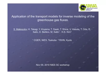
Application of the transport models for inverse modeling of the greenhouse gas fluxes greenhouse gas fluxes. S Maksyutov 1 S. Maksyutov 1 and H. Takagi, Y. Koyama, T. Saeki, V. Valsala, T. Oda, R. Saito, D. Belikov, M. Saito 1 , H-S. Kim 2 , Y.
Application of the transport models for inverse modeling of the greenhouse gas fluxes greenhouse gas fluxes. S Maksyutov 1 S. Maksyutov 1 and H. Takagi, Y. Koyama, T. Saeki, V. Valsala, T. Oda, R. Saito, D. Belikov, M. Saito 1 , H-S. Kim 2 , Y. Niwa, and R. Imasu 3 1 CGER, NIES 2 RIHN, Kyoto RIHN, Kyoto 3 CCSR, Tokyo Univ Nov 11, 2009 SC workshop
O tli Outline Improvements for the inverse model for GOSAT L4A • Terrestrial biosphere, ocean carbon cycle, atmospheric transport and fossil fuel emissions Ongoing developments Ongoing developments • Kalman smoother application with coupled transport. • Cumulus cloud mixing • • Biospheric model optimization with inversion Biospheric model optimization with inversion Summary
Tracer transport model development Model Options NIES-05 NIES-08 NIES-08 NIES-08 ¥SML¥0.5 ¥VL¥1.25 ¥VL¥0.625 ¥Pr¥2.5 Flux-form (flux version) Semi- Numerical Scheme Lagrangian 3-order van Leer 3 o de a ee 2-order Moment o de o e Resolution, deg 0.5 1.25 0.625 2.5 Number of vertical levels 47 Meteo dataset JMA/GPV dataset /G GPV meteorological dataset with v. 08 VL: Van Leer, 2 nd order resolution of 0.5 × 0.5 degrees f 0 5 × 0 5 d l ti shape function for 21 pressure levels - special v. 05 Pr: Prather, with 2 nd product for GOSAT by JMA order moments (added extra levels in LT 3 hourly (added extra levels in LT, 3 hourly v 05 SML: Semi Lagrangian v. 05 SML: Semi-Lagrangian, bilinear interpolation vs standard 6 hourly)
Tracer transport model performance NIES-08 NIES-08 NIES-08 NIES-08 NIES-05 NIES-05 Resolution Val Leer Prather SML CPU, sec 10.21 292.90 6.08 emin emin 6 22E 04 6.22E-04 1 38E 04 1.38E-04 -5.37E-03 5 37E 03 emax -2.86E-03 -3.48E-04 2.16E-03 2.5 °× 2.5 ° (2 °× 2 ° for SML) err1 -6.66E-03 -5.96E-08 6.09E-02 err2 2 1.17E-03 1 1 03 1 02 1.02E-03 03 5.08E-03 08 03 Memory, Gb 0.72 0.77 0.72 CPU, sec 55.93 1755.77 20.86 emin 1.57E-04 -5.95E-05 -0.229E-06 emax -3.66E-03 1.03E-06 0.00E+00 1.25 °× 1.25 ° (1 °× 1 ° for SML) err1 -3.50E-03 4.78E-03 1.93E-02 err2 8.94E-04 8.48E-03 9.90E-03 Memory, Gb 0.98 1.10 0.98 CPU, sec , 370.975 12683.15 82.20 emin 3.93E-05 -5.11E-06 -1.04E-07 emax -2.44E-03 -5.21E-03 7.95E-08 0.625 °× 0.625 ° (0.5 °× 0.5 ° for SML) (0 5 0 5 o S ) err1 err1 -1 75E-03 -1.75E-03 5 55E-03 5.55E-03 1.59E-02 1 59E-02 err2 6.15E-04 1.18E-04 1.74E-02 Memory, Gb 1.94 2.46 1.94
Tracer transport model: model validation Vertical mixing test: Radon simulation Radon simulation Interhemispheric mixing test: SF6 i SF6 simulation l ti
Tracer transport model: model validation Seasonal cycle of CO 2 over South Pole (-89.98;-24.80; 2810) (a) and Cold Bay in Alaska (55.20; -162.72; 25) (b) for 2008, ppmv
Land CO 2 fluxes: improved simulation seasonal cycle in atmospheric CO 2 partial column abundance in atmospheric CO 2 partial column abundance Parameter values for each ecosystem (1) li ht (1) light use efficiency for NPP ffi i f NPP (2) temperature coefficient of respiration Optimized independently for each vegetation type, completed for CASA vegetation type completed for CASA model, working on VISIT (A. Ito, M. Saito) Nakatsuka & Maksyutov Biogesci. Disc. 2009 Seasonal variation of CO partial column CO 2 partial column, with ecosystem model optimized with observations Result: observations. Result: monthly CO2 flux maps at 1x1 deg res. month
Land CO 2 fluxes: improved simulation seasonal cycle in atmospheric CO 2 partial column abundance in atmospheric CO 2 partial column abundance Seasonal variation of CO 2 vertical profile column, with VISIT ecosystem model before optimization. Red – VISIT Green – Globalview08 Plan – optimize q10 and photosynthetic capacity (and ~ 15 other Pl ti i 10 d h t th ti it ( d 15 th parameters) with inverse model
Ocean CO2 flux. 4D-var assimilation of the surface ocean pCO2 Objective: Provide ocean CO 2 flux priors for GOSAT p L4A inverse model. Physical : Oceanic TM (Valsala et al., 2008) Chemical: OCMIP-II (Watson and Orr, 2003) Biological: McKinley et al. 2004 Bi l i l M Ki l t l 2004 4D-var: Ikeda and Sasai (2002) Currents: ECCO (or GFDL) Currents: ECCO (or GFDL) DIC/pCO2 observations: LDEO database Takahashi 2009 LDEO database, Takahashi 2009 Top: assimilated pCO2 Middle: observations Bottom: assimilation - observation
Ocean fluxes: assimilation output 4D-Var assimilation of ocean CO 2 flux Period: Period: Near-Real time Completed w GFDL: 1996-2004. With ECCO: 2004-2009. Animation Multi-year assimilated air-sea CO 2 flux . Ocean currents by ECCO reanalysis (MIT ocean GCM) are y ( ) available with approximately 1 month delay . By V. Valsala et al, ICDC8, 2009
High resolution fossil fuel emissions. Using large point source data g g p Large point sources + DMSP lights Large point sources + DMSP lights and DMSP lights (1km res) produces good match at 50 km scale with high resolution bottom-up inventory by Vulcan project (K.Gurney) in US. by Oda & Maksyutov, ICDC8, 2009
Development of a coupled transport model FLEXPART 1. Objective; Coupled Model Obs. year 2005 30 Develop a new transport model 400 CO 2 (obs.) / ppm C LPDM (Fl LPDM (Flexpart) coupled with t) l d ith 20 20 CO 2 / ppm 390 NIES-TM for use in inverse 10 380 modeling 0 370 1 1 2 2 3 3 4 4 5 5 6 6 7 7 8 8 9 9 10 10 11 11 12 12 Month 2. Progress; Fig. 1. CO2 variation at Hateruma for year 2005. Model has been validated using ESRL flask and NIES using ESRL flask and NIES 30 30 1.8 1.8 continuous greenhouse gases 390 CH4 / ppm CH4 / ppm CO2 / ppm CO2 / ppm observations 1996-2007. 1.9 1.9 Coupled model 20 Obs. 380 2 2 2 370 10 3. Plan 2001/1 2001/2 2001/3 1.8 Date 30 Extend model to using GOSAT CH4 / p 2 / ppm CH4 1.9 column observations column observations NIES TM NIES TM ppm CO2 20 CO2 2 Y. Koyama et al, ICDC8 NIES TM : 2.5x2.5 10 2.1 2001/1 2001/2 2001/3 Coupled : 0.5x0.5 Date Fig. 2. CO2 and CH4 variations at Hateruma for winter season, year 2001.
Coupled transport model with 5-10 km resolution fluxes 1. Objective; 2. Progress; Test very high resolution Made comparison at Chinese simulation globally with 5-10 i l ti l b ll ith 5 10 site (data by H. Mukai et al) it (d t b H M k i t l) km emissions 3. Plan Fig. 1. Oda -5km, EDGAR-10km and CDIAC 0.5 °° Use 1 km fluxes by Oda et al, and VISIT
Inverse modeling with Lagrangian transport Obs. Obs. Prior Posterior Alert, 1996 1. Objective: Use each available observation 6 without smoothing filtering ith t thi filt i (aggregation), reduce / ppm 0 response function simulation time (5 to 10 times) time (5 to 10 times). CO 2 –6 2. Present state: Implemented fixed lag Kalman Implemented fixed lag Kalman J F M A M J J A S O smoother to use 3-hourly Obs. Month continuous observations and Prior Posterior Hateruma, 1996 flasks directly in 64 region y g 10 monthly inversion with 3-6 month time lag (Bruhwiler etal 2005), tested with 1996 data ppm CO 2 / p 0 3. Plan Complete 1980-1990 analysis in 2009 rest in 2010 in 2009, rest in 2010 –10 Y. Koyama et al, ICDC8 J F M A M J J A S O Month
Summary Improving the algorithms for regional CO2 flux estimation in global scale including: l b l l i l di • Inverse modeling with large number of observations • Fossil fuel emissions model high spatial resolution Fossil fuel emissions model, high spatial resolution • Process-based modeling of the terrestrial ecosystem fluxes • Observation-driven data assimilation system for near real-time y surface pCO2 and ocean-atmosphere flux estimation • High resolution transport modeling
Recommend
More recommend
Explore More Topics
Stay informed with curated content and fresh updates.
