Application exercise: MLR - Interpreting models and checking - PDF document

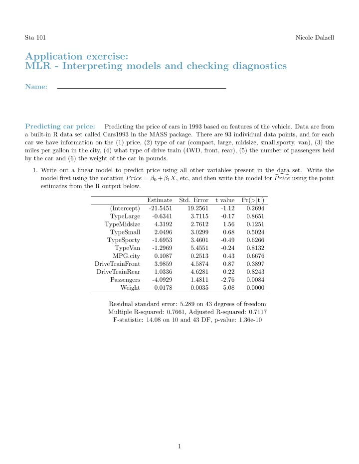
Sta 101 Nicole Dalzell Application exercise: MLR - Interpreting models and checking diagnostics Name: Predicting car price: Predicting the price of cars in 1993 based on features of the vehicle. Data are from a built-in R data set called Cars1993 in the MASS package. There are 93 individual data points, and for each car we have information on the (1) price, (2) type of car (compact, large, midsize, small,sporty, van), (3) the miles per gallon in the city, (4) what type of drive train (4WD, front, rear), (5) the number of passengers held by the car and (6) the weight of the car in pounds. 1. Write out a linear model to predict price using all other variables present in the data set. Write the model first using the notation Price = β 0 + β 1 X , etc, and then write the model for � Price using the point estimates from the R output below. Estimate Std. Error t value Pr( > | t | ) (Intercept) -21.5451 19.2561 -1.12 0.2694 TypeLarge -0.6341 3.7115 -0.17 0.8651 TypeMidsize 4.3192 2.7612 1.56 0.1251 TypeSmall 2.0496 3.0299 0.68 0.5024 TypeSporty -1.6953 3.4601 -0.49 0.6266 TypeVan -1.2969 5.4551 -0.24 0.8132 MPG.city 0.1087 0.2513 0.43 0.6676 DriveTrainFront 3.9859 4.5874 0.87 0.3897 DriveTrainRear 1.0336 4.6281 0.22 0.8243 Passengers -4.0929 1.4811 -2.76 0.0084 Weight 0.0178 0.0035 5.08 0.0000 Residual standard error: 5.289 on 43 degrees of freedom Multiple R-squared: 0.7661, Adjusted R-squared: 0.7117 F-statistic: 14.08 on 10 and 43 DF, p-value: 1.36e-10 1

2. Interpret b 0 . How many categorical variables are present in this analysis? Express the reference level for each one. 3. Interpret the point estimate for the coefficient of “typesmall” in context of the data. 4. Construct a 95% confidence interval for the slope of passengers , and interpret it in context of the data. 5. Determine which variables, if any, do not have a significant linear relationship with the outcome and should be candidates for removal from the model. If there is more than one such variable, indicate which one should be removed first, and which method you used to come to that conclusion. 2

The summary table below shows the results of the model with the driveTrain variable removed. Estimate Std. Error t value Pr( > | t | ) (Intercept) 9.5485 15.3289 0.62 0.5350 TypeLarge -0.3642 3.3735 -0.11 0.9143 TypeMidsize 2.7536 2.3716 1.16 0.2489 TypeSmall -0.9281 2.6620 -0.35 0.7282 TypeSporty -4.5070 2.9918 -1.51 0.1357 TypeVan -2.8175 4.4353 -0.64 0.5270 MPG.city -0.2320 0.2405 -0.96 0.3374 Passengers -4.2292 1.3613 -3.11 0.0026 Weight 0.0121 0.0029 4.12 0.0001 Residual standard error: 6.329 on 84 degrees of freedom Multiple R-squared: 0.608, Adjusted R-squared: 0.5707 F-statistic: 16.29 on 8 and 84 DF, p-value: 2.762e-14 (a) Using backward selection with R 2 adj , do we prefer this model to the full model? Explain. (b) Using R, and this method of model selection, determine if any other variable(s) should be removed from the model. This will be done in R as a class. 3

(c) The first car in the data set is a small car which obtains 25 mpg in the city. It has a front drive train, weights 2705 lbs and can seat 5 passengers. In the data, the price is recorded as 15.9. Calculate the residual for this observation. Does the model over or under estimate this data point? 4