Announcements Homework 2 Due 2/11 (today) at 11:59pm Electronic - - PowerPoint PPT Presentation

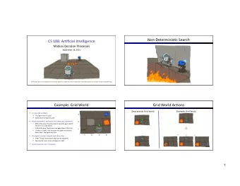
Announcements

▪ Homework 2

▪ Due 2/11 (today) at 11:59pm

▪ Electronic HW2 ▪ Written HW2

▪ Project 2

▪ Releases today ▪ Due 2/22 at 4:00pm

▪ Mini-contest 1 (optional)

▪ Due 2/11 (today) at 11:59pm

CS 188: Artificial Intelligence

How to Solve Markov Decision Processes

Instructors: Sergey Levine and Stuart Russell University of California, Berkeley

[slides adapted from Dan Klein and Pieter Abbeel http://ai.berkeley.edu.]

Example: Grid World

▪ A maze-like problem

▪ The agent lives in a grid ▪ Walls block the agent’s path

▪ Noisy movement: actions do not always go as planned

▪ 80% of the time, the action North takes the agent North ▪ 10% of the time, North takes the agent West; 10% East ▪ If there is a wall in the direction the agent would have been taken, the agent stays put

▪ The agent receives rewards each time step

▪ Small “living” reward each step (can be negative) ▪ Big rewards come at the end (good or bad)

▪ Goal: maximize sum of (discounted) rewards

Recap: MDPs

▪ Markov decision processes:

▪ States S ▪ Actions A ▪ Transitions P(s’|s,a) (or T(s,a,s’)) ▪ Rewards R(s,a,s’) (and discount γ) ▪ Start state s0

▪ Quantities:

▪ Policy = map of states to actions ▪ Utility = sum of discounted rewards ▪ Values = expected future utility from a state (max node) ▪ Q-Values = expected future utility from a q-state (chance node) a s s, a s,a,s’ ’s

Example: Racing

▪ A robot car wants to travel far, quickly ▪ Three states: Cool, Warm, Overheated ▪ Two actions: Slow, Fast ▪ Going faster gets double reward Cool Warm Overheated

Fast Fast Slow Slow 0.5 0.5 0.5 0.5 1.0 1.0 +1 +1 +1 +2 +2

• 10

Racing Search Tree

Discounting

▪ How to discount?

▪ Each time we descend a level, we multiply in the discount once

▪ Why discount?

▪ Sooner rewards probably do have higher utility than later rewards ▪ Also helps our algorithms converge

▪ Example: discount of 0.5

▪ U([1,2,3]) = 1*1 + 0.5*2 + 0.25*3 ▪ U([1,2,3]) < U([3,2,1])

Optimal Quantities

▪ The value (utility) of a state s: V*(s) = expected utility starting in s and acting optimally ▪ The value (utility) of a q-state (s,a): Q*(s,a) = expected utility starting out having taken action a from state s and (thereafter) acting optimally ▪ The optimal policy: π*(s) = optimal action from state s

a s ’s s, a

(s,a,s’) is a transition

s,a,s’

s is a state (s, a) is a q-state

[Demo: gridworld values (L9D1)]

Solving MDPs

Snapshot of Demo – Gridworld V Values

Noise = 0.2 Discount = 0.9 Living reward = 0

Snapshot of Demo – Gridworld Q Values

Noise = 0.2 Discount = 0.9 Living reward = 0

Racing Search Tree

Racing Search Tree

Racing Search Tree

▪ We’re doing way too much work with expectimax! ▪ Problem: States are repeated

▪ Idea: Only compute needed quantities once

▪ Problem: Tree goes on forever

▪ Idea: Do a depth-limited computation, but with increasing depths until change is small ▪ Note: deep parts of the tree eventually don’t matter if γ < 1

Time-Limited Values

▪ Key idea: time-limited values ▪ Define Vk(s) to be the optimal value of s if the game ends in k more time steps

▪ Equivalently, it’s what a depth-k expectimax would give from s

[Demo – time-limited values (L8D6)]

k=0

Noise = 0.2 Discount = 0.9 Living reward = 0

k=1

Noise = 0.2 Discount = 0.9 Living reward = 0

k=2

Noise = 0.2 Discount = 0.9 Living reward = 0

k=3

Noise = 0.2 Discount = 0.9 Living reward = 0

k=4

Noise = 0.2 Discount = 0.9 Living reward = 0

k=5

Noise = 0.2 Discount = 0.9 Living reward = 0

k=6

Noise = 0.2 Discount = 0.9 Living reward = 0

k=7

Noise = 0.2 Discount = 0.9 Living reward = 0

k=8

Noise = 0.2 Discount = 0.9 Living reward = 0

k=9

Noise = 0.2 Discount = 0.9 Living reward = 0

k=10

Noise = 0.2 Discount = 0.9 Living reward = 0

k=11

Noise = 0.2 Discount = 0.9 Living reward = 0

k=12

Noise = 0.2 Discount = 0.9 Living reward = 0

k=100

Noise = 0.2 Discount = 0.9 Living reward = 0

Computing Time-Limited Values

Value Iteration

Value Iteration

▪ Start with V0(s) = 0: no time steps left means an expected reward sum of zero ▪ Given vector of Vk(s) values, do one step of expectimax from each state: ▪ Repeat until convergence ▪ Complexity of each iteration: O(S2A) ▪ Theorem: will converge to unique optimal values

▪ Basic idea: approximations get refined towards optimal values ▪ Policy may converge long before values do

a Vk+1(s) s, a s,a,s’ (’Vk(s

Example: Value Iteration

0 0 0 2 1 0 3.5 2.5 0

Assume no discount!

Convergence*

▪ How do we know the Vk vectors are going to converge? ▪ Case 1: If the tree has maximum depth M, then VM holds the actual untruncated values ▪ Case 2: If the discount is less than 1

▪ Sketch: For any state Vk and Vk+1 can be viewed as depth k+1 expectimax results in nearly identical search trees ▪ The difference is that on the bottom layer, Vk+1 has actual rewards while Vk has zeros ▪ That last layer is at best all RMAX ▪ It is at worst RMIN ▪ But everything is discounted by γk that far out ▪ So Vk and Vk+1 are at most γk max|R| different ▪ So as k increases, the values converge

The Bellman Equations

How to be optimal: Step 1: Take correct first action Step 2: Keep being optimal

The Bellman Equations

▪ Definition of “optimal utility” via expectimax recurrence gives a simple one-step lookahead relationship amongst

• ptimal utility values

▪ These are the Bellman equations, and they characterize

• ptimal values in a way we’ll use over and over

a s s, a s,a,s’ ’s

Value Iteration

▪ Bellman equations characterize the optimal values: ▪ Value iteration computes them: ▪ Value iteration is just a fixed point solution method

▪ … though the Vk vectors are also interpretable as time-limited values

a V(s) s, a s,a,s’ (’V(s

Policy Methods

Policy Evaluation

Fixed Policies

▪ Expectimax trees max over all actions to compute the optimal values ▪ If we fixed some policy π(s), then the tree would be simpler – only one action per state

▪ … though the tree’s value would depend on which policy we fixed

a s s, a s,a,s’ ’s π(s) s s, π(s) s, π(s),s’ ’s Do the optimal action Do what π says to do

Utilities for a Fixed Policy

▪ Another basic operation: compute the utility of a state s under a fixed (generally non-optimal) policy ▪ Define the utility of a state s, under a fixed policy π:

Vπ(s) = expected total discounted rewards starting in s and following π

▪ Recursive relation (one-step look-ahead / Bellman equation): π(s) s s, π(s) s, π(s),s’ ’s

Example: Policy Evaluation

Always Go Right Always Go Forward

Example: Policy Evaluation

Always Go Right Always Go Forward

Policy Evaluation

▪ How do we calculate the V’s for a fixed policy π? ▪ Idea 1: Turn recursive Bellman equations into updates (like value iteration) ▪ Efficiency: O(S2) per iteration ▪ Idea 2: Without the maxes, the Bellman equations are just a linear system

▪ Solve with Matlab (or your favorite linear system solver)

π(s) s s, π(s) s, π(s),s’ ’s

Challenge question: how else can we solve this?

Policy Extraction

Computing Actions from Values

▪ Let’s imagine we have the optimal values V*(s) ▪ How should we act?

▪ It’s not obvious!

▪ We need to do a mini-expectimax (one step) ▪ This is called policy extraction, since it gets the policy implied by the values

Computing Actions from Q-Values

▪ Let’s imagine we have the optimal q-values: ▪ How should we act?

▪ Completely trivial to decide!

▪ Important lesson: actions are easier to select from q-values than values!

Policy Iteration

Problems with Value Iteration

▪ Value iteration repeats the Bellman updates: ▪ Problem 1: It’s slow – O(S2A) per iteration ▪ Problem 2: The “max” at each state rarely changes ▪ Problem 3: The policy often converges long before the values

a s s, a s,a,s’ ’s

k=0

Noise = 0.2 Discount = 0.9 Living reward = 0

k=1

Noise = 0.2 Discount = 0.9 Living reward = 0

k=2

Noise = 0.2 Discount = 0.9 Living reward = 0

k=3

Noise = 0.2 Discount = 0.9 Living reward = 0

k=4

Noise = 0.2 Discount = 0.9 Living reward = 0

k=5

Noise = 0.2 Discount = 0.9 Living reward = 0

k=6

Noise = 0.2 Discount = 0.9 Living reward = 0

k=7

Noise = 0.2 Discount = 0.9 Living reward = 0

k=8

Noise = 0.2 Discount = 0.9 Living reward = 0

k=9

Noise = 0.2 Discount = 0.9 Living reward = 0

k=10

Noise = 0.2 Discount = 0.9 Living reward = 0

k=11

Noise = 0.2 Discount = 0.9 Living reward = 0

k=12

Noise = 0.2 Discount = 0.9 Living reward = 0

k=100

Noise = 0.2 Discount = 0.9 Living reward = 0

Policy Iteration

▪ Alternative approach for optimal values:

▪ Step 1: Policy evaluation: calculate utilities for some fixed policy (not optimal utilities!) until convergence ▪ Step 2: Policy improvement: update policy using one-step look-ahead with resulting converged (but not optimal!) utilities as future values ▪ Repeat steps until policy converges

▪ This is policy iteration

▪ It’s still optimal! ▪ Can converge (much) faster under some conditions

Policy Iteration

▪ Evaluation: For fixed current policy π, find values with policy evaluation:

▪ Iterate until values converge:

▪ Improvement: For fixed values, get a better policy using policy extraction

▪ One-step look-ahead:

Comparison

▪ Both value iteration and policy iteration compute the same thing (all optimal values) ▪ In value iteration:

▪ Every iteration updates both the values and (implicitly) the policy ▪ We don’t track the policy, but taking the max over actions implicitly recomputes it

▪ In policy iteration:

▪ We do several passes that update utilities with fixed policy (each pass is fast because we consider only one action, not all of them) ▪ After the policy is evaluated, a new policy is chosen (slow like a value iteration pass) ▪ The new policy will be better (or we’re done)

▪ Both are dynamic programs for solving MDPs

Summary: MDP Algorithms

▪ So you want to….

▪ Compute optimal values: use value iteration or policy iteration ▪ Compute values for a particular policy: use policy evaluation ▪ Turn your values into a policy: use policy extraction (one-step lookahead)

▪ These all look the same!

▪ They basically are – they are all variations of Bellman updates ▪ They all use one-step lookahead expectimax fragments ▪ They differ only in whether we plug in a fixed policy or max over actions

Next Time: Reinforcement Learning!