Announcements Midterm 1 is on Monday, 7/15, during lecture time - PowerPoint PPT Presentation

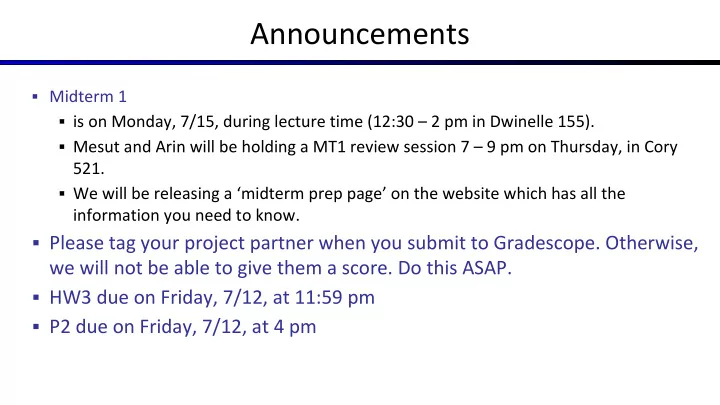
Announcements ▪ Midterm 1 ▪ is on Monday, 7/15, during lecture time (12:30 – 2 pm in Dwinelle 155). ▪ Mesut and Arin will be holding a MT1 review session 7 – 9 pm on Thursday, in Cory 521. ▪ We will be releasing a ‘midterm prep page’ on the website which has all the information you need to know. ▪ Please tag your project partner when you submit to Gradescope. Otherwise, we will not be able to give them a score. Do this ASAP. ▪ HW3 due on Friday, 7/12, at 11:59 pm ▪ P2 due on Friday, 7/12, at 4 pm

CS 188: Artificial Intelligence Probability Instructors: Aditya Baradwaj and Brijen Thananjeyan --- University of California, Berkeley [These slides were created by Dan Klein and Pieter Abbeel for CS188 Intro to AI at UC Berkeley. All CS188 materials are available at http://ai.berkeley.edu.]

Today ▪ Probability ▪ Random Variables ▪ Joint and Marginal Distributions ▪ Conditional Distribution ▪ Product Rule, Chain Rule, Bayes’ Rule ▪ Inference ▪ Independence ▪ You’ll need all this stuff A LOT for the next few weeks, so make sure you go over it now!

Inference in Ghostbusters ▪ A ghost is in the grid somewhere ▪ Sensor readings tell how close a square is to the ghost ▪ On the ghost: red ▪ 1 or 2 away: orange ▪ 3 or 4 away: yellow ▪ 5+ away: green ▪ Sensors are noisy, but we know P(Color | Distance) P(red | 3) P(orange | 3) P(yellow | 3) P(green | 3) 0.05 0.15 0.5 0.3 [Demo: Ghostbuster – no probability (L12D1) ]

Video of Demo Ghostbuster

Uncertainty ▪ General situation: ▪ Observed variables (evidence) : Agent knows certain things about the state of the world (e.g., sensor readings or symptoms) ▪ Unobserved variables : Agent needs to reason about other aspects (e.g. where an object is or what disease is present) ▪ Model : Agent knows something about how the known variables relate to the unknown variables ▪ Probabilistic reasoning gives us a framework for managing uncertain beliefs and knowledge

Random Variables ▪ A random variable is some aspect of the world about which we (may) have uncertainty ▪ R = Is it raining? ▪ T = Is it hot or cold? ▪ D = How long will it take to drive to work? ▪ L = Where is the ghost? ▪ (Technically, a random variable is a deterministic function from a possible world to some range of values.) ▪ Random variables have domains ▪ R in {true, false} (often write as {+r, -r}) ▪ T in {hot, cold} ▪ D in [0, ∞ ) ▪ L in possible locations, maybe {(0,0), (0,1), … }

Probability Distributions ▪ Associate a probability with each value ▪ Weather: ▪ Temperature: W P T P sun 0.6 hot 0.5 rain 0.1 cold 0.5 fog 0.3 meteor 0.0

Probability Distributions ▪ Unobserved random variables have distributions Shorthand notation: T P W P hot 0.5 sun 0.6 cold 0.5 rain 0.1 fog 0.3 meteor 0.0 ▪ A distribution for a discrete variable is a TABLE of OK if all domain entries are unique probabilities of values ▪ A probability (lower case value) is a single number ▪ Must have: and

Joint Distributions ▪ A joint distribution over a set of random variables: specifies a real number for each assignment (or outcome ): T W P ▪ Must obey: hot sun 0.4 hot rain 0.1 cold sun 0.2 cold rain 0.3 ▪ Size of distribution if n variables with domain sizes d? ▪ d^n. For all but the smallest distributions, impractical to write out!

Probability Models Distribution over T,W ▪ A probability model is a joint distribution over a set of random variables T W P ▪ hot sun 0.4 Probability models: ▪ (Random) variables with domains hot rain 0.1 ▪ Assignments are called outcomes ▪ Joint distributions: say whether assignments cold sun 0.2 (outcomes) are likely cold rain 0.3 ▪ Normalized: sum to 1.0 ▪ Ideally: only certain variables directly interact

Events ▪ An event E is a set of outcomes ▪ From a joint distribution, we can calculate the probability of any event T W P ▪ Probability that it’s hot AND sunny? hot sun 0.4 hot rain 0.1 ▪ Probability that it’s hot? cold sun 0.2 ▪ Probability that it’s hot OR sunny? cold rain 0.3 ▪ Typically, the events we care about are partial assignments , like P ( T=hot )

Quiz: Events ▪ P(+x, +y) ? X Y P +x +y 0.2 ▪ P(+x) ? +x -y 0.3 -x +y 0.4 -x -y 0.1 ▪ P(-y OR +x) ?

Marginal Distributions ▪ Marginal distributions are sub-tables which eliminate variables ▪ Marginalization (summing out): Combine collapsed rows by adding T P hot 0.5 T W P cold 0.5 hot sun 0.4 hot rain 0.1 cold sun 0.2 W P cold rain 0.3 sun 0.6 rain 0.4

Quiz: Marginal Distributions X P +x X Y P -x +x +y 0.2 +x -y 0.3 -x +y 0.4 Y P -x -y 0.1 +y -y

Conditional Probabilities ▪ A simple relation between joint and conditional probabilities ▪ In fact, this is taken as the definition of a conditional probability P(a,b) P(a) P(b) T W P hot sun 0.4 hot rain 0.1 cold sun 0.2 cold rain 0.3

Quiz: Conditional Probabilities ▪ P(+x | +y) ? X Y P ▪ P(-x | +y) ? +x +y 0.2 +x -y 0.3 -x +y 0.4 -x -y 0.1 ▪ P(-y | +x) ?

Conditional Distributions ▪ Conditional distributions are probability distributions over some variables given fixed values of others Conditional Distributions Joint Distribution W P T W P sun 0.8 hot sun 0.4 rain 0.2 hot rain 0.1 cold sun 0.2 cold rain 0.3 W P sun 0.4 rain 0.6

Bayes Rule

Bayes’ Rule ▪ Two ways to factor a joint distribution over two variables: That’s my rule! ▪ Dividing, we get: ▪ Why is this at all helpful? ▪ Lets us build one conditional from its reverse ▪ Often one conditional is tricky but the other one is simple ▪ Foundation of many systems we’ll see later (e.g. ASR, MT) ▪ In the running for most important AI equation!

Law of total probability ▪ An event can be split up into it’s intersection with disjoint events. ▪ Where A1, A2, ... An are mutually exclusive and exhaustive 21

Combining the two ▪ Here’s what you get when you combine Bayes’ Rule with the law of total probability: (Bayes Rule) (Law of total probability) (Bayes’ Rule)

Case Study! ▪ OJ Simpson murder trial, 1995 ▪ “Trial of the Century” ▪ OJ was suspected of murdering his wife and her friend. ▪ Mountain of evidence against him (DNA, bloody glove, history of abuse toward his wife).

Case Study ▪ Defense lawyer: Alan Dershowitz ▪ “Only one in a thousand abusive husbands eventually murder their wives.” ▪ Prosecution wasn’t able to convince the judge, and OJ was acquitted (he didn’t get charged)

Case Study ▪ Let’s define the following events: ▪ M – A wife is M urdered ▪ H – A wife is murdered by her H usband ▪ A – The husband has a history of A buse towards the wife ▪ Dershowitz’ claim: “Only one in a thousand abusive husbands eventually murder their wives.” ▪ Translates to

▪ Dershowitz’ claim: “Only one in a thousand abusive husbands eventually murder their wives.” ▪ Translates to ▪ Does anyone see the problem here? ▪ But we don’t care about P(H | A), we want P(H | A, M) ▪ Why? ▪ Since we know the wife has been murdered! 26

Case Study ▪ 27

Case Study ▪ 97% probability that OJ murdered his wife! ▪ Quite different from 0.1% ▪ Maybe if the prosecution had realized this, things would have gone differently. ▪ Moral of the story: know your conditional probability! 29

Break! ▪ Stand up and stretch ▪ Talk to your neighbors 30

Inference with Bayes’ Rule ▪ Example: Diagnostic probability from causal probability: ▪ Example: ▪ M: meningitis, S: stiff neck Example givens ▪ Note: posterior probability of meningitis still very small ▪ Note: you should still get stiff necks checked out! Why?

Quiz: Bayes’ Rule ▪ Given: D W P wet sun 0.1 W P dry sun 0.9 sun 0.8 wet rain 0.7 rain 0.2 dry rain 0.3 ▪ What is P(W | dry) ?

Ghostbusters, Revisited ▪ Let’s say we have two distributions: ▪ Prior distribution over ghost location: P(G) ▪ Let’s say this is uniform ▪ Sensor reading model: P(R | G) ▪ Given: we know what our sensors do ▪ R = reading color measured at (1,1) ▪ E.g. P(R = yellow | G=(1,1)) = 0.1 ▪ We can calculate the posterior distribution P(G|r) over ghost locations given a reading using Bayes’ rule: ▪ What about two readings? What is P ( r 1 , r 2 | g ) ?

To Normalize ▪ (Dictionary) To bring or restore to a normal condition All entries sum to ONE ▪ Procedure: ▪ Step 1: Compute Z = sum over all entries ▪ Step 2: Divide every entry by Z ▪ Example 1 ▪ Example 2 T W P T W P W P Normalize W P Normalize hot sun 20 hot sun 0.4 sun 0.2 sun 0.4 hot rain 0.1 hot rain 5 Z = 0.5 rain 0.3 rain 0.6 Z = 50 cold sun 10 cold sun 0.2 cold rain 15 cold rain 0.3

Normalization Trick ▪ A trick to get a whole conditional distribution at once: ▪ Select the joint probabilities matching the evidence ▪ Normalize the selection (make it sum to one) T W P hot sun 0.4 T R P T P hot rain 0.1 hot rain 0.1 hot 0.25 Normalize Select cold sun 0.2 cold rain 0.3 cold 0.75 cold rain 0.3 ▪ Why does this work? Sum of selection is P(evidence)! (P(r), here)