Announcements Monday, August 27 Make sure your poll scores are in - PowerPoint PPT Presentation

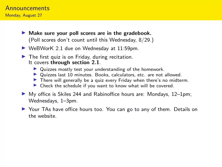
Announcements Monday, August 27 ◮ Make sure your poll scores are in the gradebook. (Poll scores don’t count until this Wednesday, 8/29.) ◮ WeBWorK 2.1 due on Wednesday at 11:59pm. ◮ The first quiz is on Friday, during recitation. It covers through section 2.1 . ◮ Quizzes mostly test your understanding of the homework. ◮ Quizzes last 10 minutes. Books, calculators, etc. are not allowed. ◮ There will generally be a quiz every Friday when there’s no midterm. ◮ Check the schedule if you want to know what will be covered. ◮ My office is Skiles 244 and Rabinoffice hours are: Mondays, 12–1pm; Wednesdays, 1–3pm. ◮ Your TAs have office hours too. You can go to any of them. Details on the website.

Solving Systems of Equations Example Solve the system of equations x + 2 y + 3 z = 6 2 x − 3 y + 2 z = 14 3 x + y − z = − 2 This is the kind of problem we’ll talk about for the first half of the course. ◮ A solution is a list of numbers x , y , z , . . . that makes all of the equations true. ◮ The solution set is the collection of all solutions. ◮ Solving the system means finding the solution set in a “parameterized” form. What is a systematic way to solve a system of equations?

Solving Systems of Equations Example Solve the system of equations x + 2 y + 3 z = 6 2 x − 3 y + 2 z = 14 3 x + y − z = − 2 What strategies do you know? ◮ Substitution ◮ Elimination Both are perfectly valid, but only elimination scales well to large numbers of equations.

Solving Systems of Equations Example Solve the system of equations x + 2 y + 3 z = 6 2 x − 3 y + 2 z = 14 3 x + y − z = − 2 Elimination method: in what ways can you manipulate the equations? ◮ Multiply an equation by a nonzero number. (scale) ◮ Add a multiple of one equation to another. (replacement) ◮ Swap two equations. (swap)

Solving Systems of Equations Example Solve the system of equations x + 2 y + 3 z = 6 2 x − 3 y + 2 z = 14 3 x + y − z = − 2 − 3 x − 6 y − 9 z = − 18 Multiply first by − 3 2 x − 3 y + 2 z = 14 3 x + y − z = − 2 − 3 x − 6 y − 9 z = − 18 Add first to third 2 x − 3 y + 2 z = 14 − 5 y − 10 z = − 20 Now I’ve eliminated x from the last equation! . . . but there’s a long way to go still. Can we make our lives easier?

Solving Systems of Equations Better notation It sure is a pain to have to write x , y , z , and = over and over again. Matrix notation: write just the numbers, in a box, instead! x + 2 y + 3 z = 6   1 2 3 6 becomes 2 x − 3 y + 2 z = 14 2 − 3 2 14   3 1 − 1 − 2 3 x + y − z = − 2 This is called an (augmented) matrix . Our equation manipulations become elementary row operations : ◮ Multiply all entries in a row by a nonzero number. (scale) ◮ Add a multiple of each entry of one row to the corresponding entry in another. (row replacement) ◮ Swap two rows. (swap)

Row Operations Example Solve the system of equations x + 2 y + 3 z = 6 2 x − 3 y + 2 z = 14 3 x + y − z = − 2 Start:   1 2 3 6 2 − 3 2 14   3 1 − 1 − 2 Goal: we want our elimination method to eventually produce a system of equations like x = A  1 0 0  A or in matrix form, 0 1 0 y = B B   0 0 1 C z = C So we need to do row operations that make the start matrix look like the end one. Strategy (preliminary): fiddle with it so we only have ones and zeros. [animated]

Row Operations Continued  1 2 3 6   1 2 3 6  R 2 = R 2 − 2 R 1 2 − 3 2 14 0 − 7 − 4 2     3 1 − 1 − 2 3 1 − 1 − 2   1 2 3 6 R 3 = R 3 − 3 R 1 0 − 7 − 4 2 We want these to be zero.   0 − 5 − 10 − 20 So we subract multiples of the first row.     1 2 3 6 1 2 3 6 R 2 ← → R 3 0 − 7 − 4 2 0 − 5 − 10 − 20     0 − 5 − 10 − 20 0 − 7 − 4 2   1 2 3 6 R 2 = R 2 ÷ − 5 0 1 2 4   We want these to be zero. 0 − 7 − 4 2 It would be nice if this were a 1.  1 0 − 1 − 2  R 1 = R 1 − 2 R 2 We could divide by − 7, but that 0 1 2 4 would produce ugly fractions.   0 − 7 − 4 2 Let’s swap the last two rows first.   1 0 − 1 − 2 R 3 = R 3 + 7 R 2 0 1 2 4   0 0 10 30

Row Operations Continued  1 0 − 1 − 2   1 0 − 1 − 2  R 3 = R 3 ÷ 10 0 1 2 4 0 1 2 4     0 0 10 30 0 0 1 3   1 0 0 1 R 1 = R 1 + R 3 0 1 2 4 We want these to be zero.   0 0 1 3 Let’s make this a 1 first.   1 0 0 1 R 2 = R 2 − 2 R 3 0 1 0 − 2   0 0 1 3 = 1 x translates into = − 2 y z = 3 Success! Check: x + 2 y + 3 z = 6 1 + 2 · ( − 2) + 3 · 3 = 6 substitute solution 3 = − 2 � 2 x − 3 y + 2 z = 14 2 · 1 − 3 · ( − 2) + 2 · 3 = 14 3 x + z = − 2 y − 3 · 1 + ( − 2) −

Row Equivalence Important The process of doing row operations to a matrix does not change the solution set of the corresponding linear equations! Definition Two matrices are called row equivalent if one can be obtained from the other by doing some number of elementary row operations. So the linear equations of row-equivalent matrices have the same solution set .

A Bad Example Example Solve the system of equations x + y = 2 3 x + 4 y = 5 4 x + 5 y = 9 Let’s try doing row operations: [interactive row reducer]     1 1 2 1 1 2 R 2 = R 2 − 3 R 1 First clear these by 3 4 5 0 1 − 1     subtracting multiples 4 5 9 4 5 9 of the first row.  1 1 2  R 3 = R 3 − 4 R 1 0 1 − 1   0 1 1     1 1 2 1 1 2 R 3 = R 3 − R 2 0 1 − 1 0 1 − 1 Now clear this by     0 1 1 0 0 2 subtracting the second row.

A Bad Example Continued  1 1 2  x + y = 2 translates into 0 1 − 1 y = − 1   0 0 2 0 = 2 In other words, the original equations x + y = 2 x + y = 2 3 x + 4 y = 5 have the same solutions as y = − 1 4 x + 5 y = 9 0 = 2 But the latter system obviously has no solutions (there is no way to make them all true), so our original system has no solutions either. Definition A system of equations is called inconsistent if it has no solution. It is consistent otherwise.

Section 2.2 Row Reduction

Row Echelon Form Let’s come up with an algorithm for turning an arbitrary matrix into a “solved” matrix. What do we mean by “solved”? A matrix is in row echelon form if 1. All zero rows are at the bottom. 2. Each leading nonzero entry of a row is to the right of the leading entry of the row above. 3. Below a leading entry of a row, all entries are zero . Picture:   ⋆ ⋆ ⋆ ⋆ ⋆ ⋆ = any number 0 ⋆ ⋆ ⋆ ⋆     0 0 0 ⋆ = any nonzero number ⋆ ⋆   0 0 0 0 0 Definition A pivot ⋆ is the first nonzero entry of a row of a matrix. A pivot column is a column containing a pivot of a matrix in row echelon form .

Reduced Row Echelon Form A matrix is in reduced row echelon form if it is in row echelon form, and in addition, 4. The pivot in each nonzero row is equal to 1. 5. Each pivot is the only nonzero entry in its column. Picture:   1 0 0 ⋆ ⋆ ⋆ = any number 0 1 0 ⋆ ⋆     0 0 0 1 1 = pivot ⋆   0 0 0 0 0 Note: Echelon forms do not care whether or not a column is augmented. Just ignore the vertical line. Question Can every matrix be put into reduced row echelon form only using row operations? Answer: Yes! Stay tuned.

Reduced Row Echelon Form Continued Why is this the “solved” version of the matrix?   1 0 0 1 0 1 0 − 2   0 0 1 3 is in reduced row echelon form. It translates into x = 1 y = − 2 z = 3, which is clearly the solution. But what happens if there are fewer pivots than rows?   1 2 0 1 0 0 1 3   0 0 0 0 . . . parametrized solution set (later).

Poll Poll Which of the following matrices are in reduced row echelon form? � 1 � 0 0 � 0 0 � A. B. 0 2 0 0 0   0 1   � � � � C. D. 0 1 0 0 E. 0 1 8 0   0   0 � 1 � 17 0 F. 0 0 1 Answer: B, D, E, F. Note that A is in row echelon form though.

Summary ◮ Solving a system of equations means producing all values for the unknowns that make all the equations true simultaneously. ◮ It is easier to solve a system of linear equations if you put all the coefficients in an augmented matrix . ◮ Solving a system using the elimination method means doing elementary row operations on an augmented matrix. ◮ Two systems or matrices are row-equivalent if one can be obtained from the other by doing a sequence of elementary row operations. Row-equivalent systems have the same solution set . ◮ A linear system with no solutions is called inconsistent . ◮ The (reduced) row echelon form of a matrix is its “solved” row-equivalent version.