Announcements Monday, November 06 This weeks quiz: covers Sections - PowerPoint PPT Presentation
Announcements Monday, November 06 This weeks quiz: covers Sections 5.1 and 5.2 Midterm 3, on November 17th (next Friday) Exam covers: Sections 3.1,3.2,5.1,5.2,5.3 and 5.5 Section 5.3 Diagonalization Motivation: Difference
Announcements Monday, November 06 ◮ This week’s quiz: covers Sections 5.1 and 5.2 ◮ Midterm 3, on November 17th (next Friday) ◮ Exam covers: Sections 3.1,3.2,5.1,5.2,5.3 and 5.5
Section 5.3 Diagonalization
Motivation: Difference equations Now do multiply matrices Many real-word (linear algebra problems): ◮ Start with a given situation ( v 0 ) and ◮ want to know what happens after some time (iterate a transformation): v n = Av n − 1 = . . . = A n v 0 . ◮ Ultimate question: what happens in the long run (find v n as n → ∞ ) Old Example Recall our example about rabbit populations : using eigenvectors was easier than matrix multiplications, but . . . ◮ Taking powers of diagonal matrices is easy! ◮ Working with diagonalizable matrices is also easy.
Powers of Diagonal Matrices If D is diagonal Then D n is also diagonal, the diagonal entries of D n are the nth powers of the diagonal entries of D
Powers of Matrices that are Similar to Diagonal Ones When is A is not diagonal? Example � 1 � 2 . Compute A n . Using that Let A = − 1 4 � 2 � 2 � � 1 0 A = PDP − 1 where P = and D = . 1 1 0 3 From the first expression: A 2 = A 3 = . . . A n = Plug in P and D : A n =
Diagonalizable Matrices Definition An n × n matrix A is diagonalizable if it is similar to a diagonal matrix: A = PDP − 1 for D diagonal. Important 0 · · · 0 d 11 0 d 22 · · · 0 If A = PDP − 1 for D = then . . . ... . . . . . . 0 0 · · · d nn d k 0 · · · 0 11 d k 0 · · · 0 22 A k = PD K P − 1 = P P − 1 . . . . ... . . . . . . d k 0 0 · · · nn So diagonalizable matrices are easy to raise to any power .
Diagonalization The Diagonalization Theorem An n × n matrix A is diagonalizable if and only if A has n linearly independent eigenvectors . In this case, A = PDP − 1 for λ 1 0 · · · 0 | | | 0 λ 2 · · · 0 P = · · · D = , v 1 v 2 v n . . . ... . . . . . . | | | 0 0 · · · λ n where v 1 , v 2 , . . . , v n are linearly independent eigenvectors, and λ 1 , λ 2 , . . . , λ n are the corresponding eigenvalues (in the same order). Important ◮ If A has n distinct eigenvalues then A is diagonalizable . ◮ If A is diagonalizable matrix it need not have n distinct eigenvalues though.
Diagonalization Example � 1 2 � Problem: Diagonalize A = . − 1 4
Diagonalization Example 2 4 − 3 0 Problem: Diagonalize A = 2 − 1 0 . 1 − 1 1
Diagonalization Example 2, continued In this case: there are 3 linearly independent eigenvectors and only 2 distinct eigenvalues.
Diagonalization Procedure How to diagonalize a matrix A : 1. Find the eigenvalues of A using the characteristic polynomial. 2. Compute a basis B λ for each λ -eigenspace of A . 3. If there are fewer than n total vectors in the union of all of the eigenspace bases B λ , then the matrix is not diagonalizable. 4. Otherwise , the n vectors v 1 , v 2 , . . . , v n in your eigenspace bases are linearly independent, and A = PDP − 1 for λ 1 0 · · · 0 | | | 0 λ 2 · · · 0 P = · · · and D = , v 1 v 2 v n . . . ... . . . . . . | | | 0 0 · · · λ n where λ i is the eigenvalue for v i .
Diagonalization A non-diagonalizable matrix � 1 1 � Problem: Show that A = is not diagonalizable . 0 1 Conclusion: � 1 � ◮ All eigenvectors of A are multiples of . 0 ◮ So A has only one linearly independent eigenvector ◮ If A was diagonalizable, there would be two linearly independent eigenvectors !
Poll
Non-Distinct Eigenvalues Definition Let λ be an eigenvalue of a square matrix A . The geometric multiplicity of λ is the dimension of the λ -eigenspace . Theorem Let λ be an eigenvalue of a square matrix A . Then 1 ≤ (the geometric multiplicity of λ ) ≤ (the algebraic multiplicity of λ ) . ◮ Note: If λ is an eigenvalue, then the λ -eigenspace has dimension at least 1. ◮ ...but it might be smaller than what the characteristic polynomial suggests. The intuition/visualisation is beyond the scope of this course .
Non-Distinct Eigenvalues (Good) examples From previous exercises we know: Example 4 − 3 0 has characteristic polynomial The matrix A = 2 − 1 0 1 − 1 1 f ( λ ) = − ( λ − 1) 2 ( λ − 2) . � 1 2 � The matrix B = has characteristic polynomial − 1 4 f ( λ ) = (1 − λ )(4 − λ ) + 2 = ( λ − 2)( λ − 3) . Matrix A Geom. M. Alg. M. Matrix B Geom. M. Alg. M. λ = 1 2 2 λ = 2 1 1 λ = 2 1 1 λ = 3 1 1 Thus, both matrices are diagonalizable .
Non-Distinct Eigenvalues (Bad) example Example � 1 � 1 has characteristic polynomial f ( λ ) = ( λ − 1) 2 . The matrix A = 0 1 We showed before that the 1 -eigenspace has dimension 1 and A was not diagonalizable . Eigenvalue Geometric Algebraic λ = 1 1 2 The Diagonalization Theorem (Alternate Form) Let A be an n × n matrix. The following are equivalent: 1. A is diagonalizable . 2. The sum of the geometric multiplicities of the eigenvalues of A equals n . 3. The sum of all algebraic multiplicities is n . And for each eigenvalue, the geometric and algebraic multiplicity are equal.
Applications to Difference Equations � 1 � 0 Let D = . 0 1 / 2 Start with a vector v 0 , and let v 1 = Dv 0 , v 2 = Dv 1 , . . . , v n = D n v 0 . Question: What happens to the v i ’s for different starting vectors v 0 ? ◮ the x -coordinate equals the initial coordinate, ◮ the y -coordinate gets halved every time.
Applications to Difference Equations Picture � 1 � a � a � 0 � � a � � D = = 0 1 / 2 b / 2 b b v 0 e 2 v 1 v 2 e 1 v 3 1-eigenspace v 4 1 / 2-eigenspace So all vectors get “collapsed into the x-axis” , which is the 1-eigenspace.
Applications to Difference Equations More complicated example � 3 / 4 1 / 4 � Let A = . 1 / 4 3 / 4 Start with a vector v 0 , and let v 1 = Av 0 , v 2 = Av 1 , . . . , v n = A n v 0 . Question: What happens to the v i ’s for different starting vectors v 0 ? Matrix Powers: This is a diagonalization question. Bottom line: A = PDP − 1 for � 1 � 1 � � 1 0 P = D = . 1 − 1 0 1 / 2 Hence v n = PD n P − 1 v 0 .
Applications to Difference Equations Picture of the more complicated example A n = PD n P − 1 acts on the usual coordinates of v 0 in the same way that D n acts on the B -coordinates, where B = { w 1 , w 2 } . 1 / 2-eigenspace 1-eigenspace v 0 w 1 v 1 v 2 v 3 w 2 v 4 So all vectors get “collapsed into the 1 -eigenspace” .
Extra: Proof Diagonalization Theorem Why is the Diagonalization Theorem true?
Recommend
More recommend
Explore More Topics
Stay informed with curated content and fresh updates.


