Announcements Class is 170. Matlab Grader homework, 1 and 2 (of - PowerPoint PPT Presentation

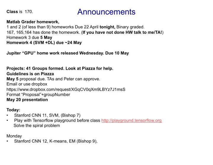
Announcements Class is 170. Matlab Grader homework, 1 and 2 (of less than 9) homeworks Due 22 April tonight, Binary graded. 167, 165,164 has done the homework. ( If you have not done HW talk to me/TA! ) Homework 3 due 5 May Homework 4 (SVM +DL) due ~24 May Jupiter “GPU” home work released Wednesday. Due 10 May Projects: 41 Groups formed. Look at Piazza for help. Guidelines is on Piazza May 5 proposal due. TAs and Peter can approve. Email or use dropbox https://www.dropbox.com/request/XGqCV0qXm9LBYz7J1msS Format “Proposal”+groupNumber May 20 presentation Today: • Stanford CNN 11, SVM, (Bishop 7) • Play with Tensorflow playground before class http://playground.tensorflow.org Solve the spiral problem Monday • Stanford CNN 12, K-means, EM (Bishop 9),

Projects • 3-4 person groups preferred • Deliverables: Poster, Report & main code ( plus proposal, midterm slide ) • Topics your own or chose form suggested topics. Some physics inspired . • April 26 groups due to TA. • 41 Groups formed. Look at Piazza for help. • Guidelines is on Piazza • May 5 proposal due. TAs and Peter can approve. Email or use dropbox Format “Proposal”+groupNumber https://www.dropbox.com/request/XGqCV0qXm9LBYz7J1msS • May 20 Midterm slide presentation. Presented to a subgroup of class. • June 5 final poster. Upload June ~3 • Report and code due Saturday 15 June.

Confusion matrix/Wikipedia If a classification system has been trained to distinguish between cats, dogs and rabbits, a confusion matrix will summarize the test results. Assuming a sample of 27 animals — 8 cats, 6 dogs, and 13 rabbits, the confusion matrix could look like the table below:

Let us define an experiment from P positive instances and N negative instances for some condition. The four outcomes can be formulated in a 2×2 confusion matrix , as follows: Recall

ROC curve (receiver operating charateristic)

Other Computer Vision Tasks Instance Semantic Classification Object Segmentation Segmentation + Localization Detection GRASS , CAT , CAT DOG , DOG , CAT DOG , DOG , CAT TREE , SKY Multiple Object No objects, just pixels Single Object This image is CC0 public domain Lecture 11 - May 10, 2017 Fei-Fei Li & Justin Johnson & Serena Yeung 17

Semantic Segmentation Idea: Fully Convolutional Upsampling : Design network as a bunch of convolutional layers, with Downsampling : Unpooling or strided downsampling and upsampling inside the network! Pooling, strided transpose convolution convolution Med-res: Med-res: D 2 x H/4 x W/4 D 2 x H/4 x W/4 Low-res: D 3 x H/4 x W/4 Input: High-res: High-res: Predictions: 3 x H x W D 1 x H/2 x W/2 D 1 x H/2 x W/2 H x W Long, Shelhamer, and Darrell, “Fully Convolutional Networks for Semantic Segmentation”, CVPR 2015 Noh et al, “Learning Deconvolution Network for Semantic Segmentation”, ICCV 2015 Lecture 11 - May 10, 2017 Fei-Fei Li & Justin Johnson & Serena Yeung 44

In-Network upsampling: “Unpooling” “Bed of Nails” Nearest Neighbor 1 0 2 0 1 1 2 2 1 2 1 2 0 0 0 0 1 1 2 2 3 4 3 4 3 0 4 0 3 3 4 4 0 0 0 0 3 3 4 4 Input: 2 x 2 Output: 4 x 4 Input: 2 x 2 Output: 4 x 4 In-Network upsampling: “Max Unpooling” Max Pooling Max Unpooling Remember which element was max! Fei-Fei Li & Justin Johnson & Serena Yeung Lecture 11 - May 10, 2017 Use positions from 26 pooling layer 0 0 2 0 1 2 6 3 1 2 … 0 1 0 0 3 5 2 1 5 6 3 4 0 0 0 0 1 2 2 1 7 8 Rest of the network 3 0 0 4 7 3 4 8 Input: 2 x 2 Output: 4 x 4 Input: 4 x 4 Output: 2 x 2 Corresponding pairs of downsampling and upsampling layers Lecture 11 - May 10, 2017 Fei-Fei Li & Justin Johnson & Serena Yeung 27

Learnable Upsampling: Transpose Convolution Recall: Normal 3 x 3 convolution, stride 2 pad 1 Filter moves 2 pixels in the input for every one Dot product pixel in the output between filter and input Stride gives ratio between movement in input and output Learnable Upsampling: Transpose Convolution Input: 4 x 4 Output: 2 x 2 Sum where 3 x 3 transpose convolution, stride 2 pad 1 Other names: Fei-Fei Li & Justin Johnson & Serena Yeung Lecture 11 - 33 May 10, 2017 output overlaps -Deconvolution (bad) -Upconvolution -Fractionally strided convolution Filter moves 2 pixels in -Backward strided the output for every one convolution Input gives pixel in the input weight for filter Stride gives ratio between movement in output and input Input: 2 x 2 Output: 4 x 4 Fei-Fei Li & Justin Johnson & Serena Yeung Lecture 11 - May 10, 2017 38

Transpose Convolution: 1D Example Output Input Filter Output contains ax copies of the filter weighted by the x ay input, summing at where at overlaps in a the output y az + bx b Need to crop one z pixel from output to by make output exactly 2x input bz Fei-Fei Li & Justin Johnson & Serena Yeung Lecture 11 - 39 May 10, 2017

Convolution as Matrix Multiplication (1D Example) We can express convolution in Convolution transpose multiplies by the terms of a matrix multiplication transpose of the same matrix: 5/1/2019 comparison convolution correlation When stride=1, convolution transpose is Example: 1D conv, kernel just a regular convolution (with different size=3, stride=1, padding=1 Convolution Cross-correlation Autocorrelation padding rules) f f f Lecture 11 - May 10, 2017 Fei-Fei Li & Justin Johnson & Serena Yeung 41 g g g f ∗ g g ⋆ f f ⋆ f g ∗ f f ⋆ g g ⋆ g https://upload.wikimedia.org/wikipedia/commons/2/21/Comparison_convolution_correlation.svg 1/1

Convolution as Matrix Multiplication (1D Example) We can express convolution in Convolution transpose multiplies by the terms of a matrix multiplication transpose of the same matrix: Example: 1D conv, kernel When stride>1, convolution transpose is size=3, stride=2, padding=1 no longer a normal convolution! Lecture 11 - May 10, 2017 Fei-Fei Li & Justin Johnson & Serena Yeung 43

Object Detection as Classification: Sliding Window Apply a CNN to many different crops of the image, CNN classifies each crop as object or background Dog? NO Cat? YES Background? NO Problem: Need to apply CNN to huge number of locations and scales, very computationally expensive! Region Proposals Lecture 11 - May 10, 2017 Fei-Fei Li & Justin Johnson & Serena Yeung 61 ● Find “blobby” image regions that are likely to contain objects ● Relatively fast to run; e.g. Selective Search gives 1000 region proposals in a few seconds on CPU Alexe et al, “Measuring the objectness of image windows”, TPAMI 2012 Uijlings et al, “Selective Search for Object Recognition”, IJCV 2013 Cheng et al, “BING: Binarized normed gradients for objectness estimation at 300fps”, CVPR 2014 Zitnick and Dollar, “Edge boxes: Locating object proposals from edges”, ECCV 2014 Fei-Fei Li & Justin Johnson & Serena Yeung Lecture 11 - 62 May 10, 2017

Image by MIT OpenCourseWare. 4 5 |{z} |{z} |{z} |{z} Kernels We might want to consider something more complicated than a linear model: � � ⇥ x (1)2 , x (2)2 , x (1) x (2) ⇤ Example 1 : [ x (1) , x (2) ] → Φ [ x (1) , x (2) ] = Information unchanged, but now we have a linear classifier on the transformed points. With the kernel trick, we just need kernel Input Space Feature Space 𝑙 𝒃, 𝒄 = 𝜲(𝒃) ) 𝜲(𝒄) Image by MIT OpenCourseWare.

Dual representation, Sec 6.2 Primal problem: min 𝐹(𝒙) 𝒙 = 𝒙 ) 𝒚 < − 𝑢 < 2 + B 𝐹 = 9 B : 𝒙 2 = 𝒀𝒙 − 𝒖 : : + : ∑ < : 𝒙 2 Solution 𝒙 = 𝒀 E 𝒖 = (𝒀 ) 𝒀 + 𝜇𝑱 𝑵 ) J𝟐 𝒀 ) 𝒖 = 𝒀 ) (𝒀𝒀 𝑼 + 𝜇𝑱 𝑶 ) J9 𝒖 = 𝒀 ) (𝑳 + 𝜇𝑱 𝑶 ) J9 𝒖 = 𝒀 ) 𝒃 The kernel is 𝐋 = 𝒀𝒀 𝑼 Dual representation is : min 𝐹(𝒃) 𝒃 = 𝒙 ) 𝒚 < − 𝑢 < 2 + B 𝐹 = 9 : + B : 𝒙 2 = 𝑳𝒃 − 𝒖 : : 𝒃 ) 𝑳𝒃 : ∑ < Prediction = 𝑏 < 𝒚 < = 𝑏 < 𝑙(𝒚 < , 𝒚) 𝑧 = 𝒙 ) 𝒚 = 𝒃 ) 𝒀𝒚 = ∑ < ) 𝒚 = ∑ <

Dual representation, Sec 6.2 Prediction = 𝑏 < 𝒚 < = 𝑏 < 𝑙(𝒚 < , 𝒚) 𝑧 = 𝒙 ) 𝒚 = 𝒃 ) 𝒀𝒚 = ∑ < ) 𝒚 = ∑ < • Often a is sparse (… Support vector machines ) • We don’t need to know x or 𝝌 𝒚 . 𝑲𝒗𝒕𝒖 𝒖𝒊𝒇 𝑳𝒇𝒔𝒐𝒇𝒎 : + 𝜇 2 𝒃 ) 𝑳𝒃 𝐹 𝒃 = 𝑳𝒃 − 𝒖 :

Lecture 10 Support Vector Machines Non Bayesian! Features: • Kernel • Sparse representations • Large margins

Regularize for plausibility • Which one is best? • We maximize the margin

Regularize for plausibility

Support Vector Machines • The line that maximizes the minimum margin is a good bet. – The model class of “hyper-planes with a margin m ” has a low VC dimension if m is big. • This maximum-margin separator is determined by a subset of the datapoints. – Datapoints in this subset are called “ support vectors ”. – It is useful computationally if only few datapoints are support vectors, because the support vectors decide which side of The support vectors are the separator a test case is on. indicated by the circles around them.

Lagrange multiplier (Bishop App E) max 𝑔 𝑦 subject to 𝑕 𝑦 = 0 Taylor expansion 𝑕 𝒚 + 𝜻 = 𝑕 𝒚 + 𝝑 ) ∇ 𝑕 𝒚 𝑀 𝑦, 𝜇 = 𝑔 𝑦 + 𝜇𝑕(𝑦)