Announcements Course survey See link on Piazza Fitting: Please - PDF document

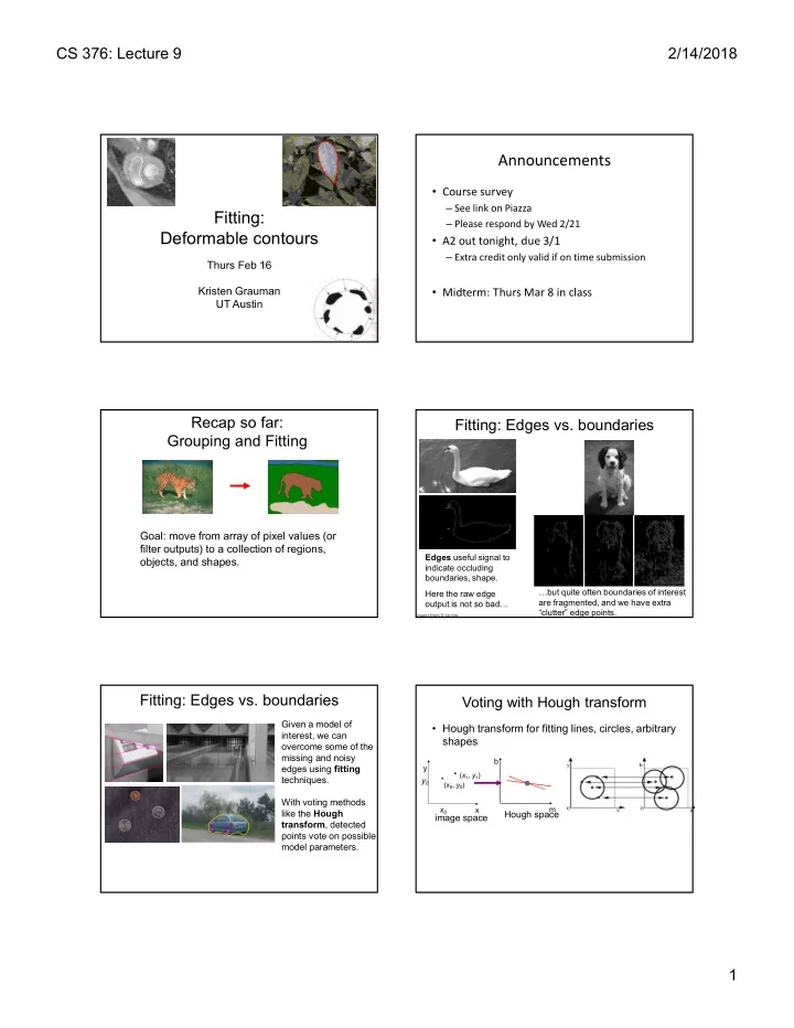
CS 376: Lecture 9 2/14/2018 Announcements • Course survey – See link on Piazza Fitting: – Please respond by Wed 2/21 Deformable contours • A2 out tonight, due 3/1 – Extra credit only valid if on time submission Thurs Feb 16 Kristen Grauman • Midterm: Thurs Mar 8 in class UT Austin Recap so far: Fitting: Edges vs. boundaries Grouping and Fitting Goal: move from array of pixel values (or filter outputs) to a collection of regions, Edges useful signal to objects, and shapes. indicate occluding boundaries, shape. …but quite often boundaries of interest Here the raw edge are fragmented, and we have extra output is not so bad… “clutter” edge points. Images from D. Jacobs Fitting: Edges vs. boundaries Voting with Hough transform Given a model of • Hough transform for fitting lines, circles, arbitrary interest, we can shapes overcome some of the missing and noisy b edges using fitting y ( x 1 , y 1 ) techniques. y 0 ( x 0 , y 0 ) With voting methods x 0 x m like the Hough Hough space image space transform , detected points vote on possible model parameters. 1

CS 376: Lecture 9 2/14/2018 Generalized Hough for object detection Recall: Generalized Hough Transform • Instead of indexing displacements by gradient • What if we want to detect arbitrary shapes? orientation, index by matched local patterns. Intuition: Displacement x vectors x x Ref. point “visual codeword” with x displacement vectors x Model image Novel image Vote space training image B. Leibe, A. Leonardis, and B. Schiele, Combined Object Categorization and Segmentation with an Implicit Shape Model, ECCV Workshop on Statistical Learning in Computer Vision 2004 Source: L. Lazebnik Generalized Hough for object detection Now • Instead of indexing displacements by gradient orientation, index by “visual codeword” • Fitting an arbitrary shape with “active” deformable contours test image B. Leibe, A. Leonardis, and B. Schiele, Combined Object Categorization and Segmentation with an Implicit Shape Model, ECCV Workshop on Statistical Learning in Computer Vision 2004 Source: L. Lazebnik Deformable contours Deformable contours a.k.a. active contours, snakes a.k.a. active contours, snakes Given : initial contour (model) near desired object Given : initial contour (model) near desired object Goal : evolve the contour to fit exact object boundary Main idea : elastic band is iteratively adjusted so as to • be near image positions with high gradients, and • satisfy shape “preferences” or contour priors [Snakes: Active contour models, Kass, Witkin, & Terzopoulos, ICCV1987] [Snakes: Active contour models, Kass, Witkin, & Terzopoulos, ICCV1987] Figure credit: Yuri Boykov Figure credit: Yuri Boykov 2

CS 376: Lecture 9 2/14/2018 Deformable contours: intuition Deformable contours vs. Hough Like generalized Hough transform, useful for shape fitting; but initial intermediate final Hough Deformable contours Rigid model shape Prior on shape types, but shape iteratively adjusted ( deforms ) Single voting pass can detect multiple instances Requires initialization nearby One optimization “pass” to fit a single contour Image from http://www.healthline.com/blogs/exercise_fitness/uploaded_images/HandBand2-795868.JPG Why do we want to fit Why do we want to fit deformable shapes? deformable shapes? • Non-rigid, deformable objects can change their shape over • Some objects have similar basic form but time, e.g. lips, some variety in the contour shape. hands… Figure from Kass et al. 1987 Why do we want to fit Why do we want to fit deformable shapes? deformable shapes? • Non-rigid, deformable objects can change their shape over time, e.g. lips, hands… • Non-rigid, deformable objects can change their shape over time. Figure credit: Julien Jomier 3

CS 376: Lecture 9 2/14/2018 Representation Aspects we need to consider • We’ll consider a discrete representation of the contour, • Representation of the contours consisting of a list of 2d point positions (“vertices”). • Defining the energy functions   ( x , y ), ( x 0 y , ) – External i i i 0 – Internal   i 0 , 1 , , n 1  for • Minimizing the energy function ( x 19 y , ) 19 • Extensions: – Tracking • At each iteration, we’ll have the – Interactive segmentation option to move each vertex to another nearby location (“state”). Energy function Fitting deformable contours How should we adjust the current contour to form the new The total energy (cost) of the current snake is contour at each iteration? defined as: • Define a cost function (“energy” function) that says how   E E E good a candidate configuration is. total internal external • Seek next configuration that minimizes that cost function. Internal energy: encourage prior shape preferences: e.g., smoothness, elasticity, particular known shape. External energy (“image” energy): encourage contour to fit on places where image structures exist, e.g., edges. A good fit between the current deformable contour initial intermediate final and the target shape in the image will yield a low value for this cost function. External energy: intuition External image energy • Measure how well the curve matches the image data How do edges affect “snap” of • “Attract” the curve toward different image features rubber band? – Edges, lines, texture gradient, etc. Think of external energy from image as gravitational pull towards areas of high contrast Magnitude of gradient - (Magnitude of gradient) 2  2 G ( I ) G ( I )   x y  2  2 G ( I ) G ( I ) x y 4

CS 376: Lecture 9 2/14/2018 External image energy Internal energy: intuition • Gradient images and G x ( x , y ) G y ( x , y ) • External energy at a point on the curve is:     2   2 E ( ) ( | G ( ) | | G ( ) | ) What are the underlying And in this one? external x y boundaries in this fragmented • External energy for the whole curve: edge image? n  1    2  2 E | G ( x , y ) | | G ( x , y ) | external x i i y i i i  0 Internal energy: intuition Internal energy For a continuous curve, a common internal energy term A priori , we want to favor smooth shapes, contours with is the “bending energy”. low curvature , contours similar to a known shape , etc. to balance what is actually observed (i.e., in the gradient At some point v(s) on the curve, this is: image). 2  2 2  d d E internal (  ( s ))     2 ds d s Tension, Stiffness, Elasticity Curvature Example: compare curvature Internal energy 2       • For our discrete representation, E curvature v ( ) 2 i i  1 i i  1           ( x 2 x x ) 2 ( y 2 y y ) 2 ( x , y ) i 0 n 1  …     i 1 i i 1 i 1 i i 1 i i i (2,5) 2   d d                v   ( ) ( ) 2     i  1 i 2 i 1 i i i 1 i 1 i i 1 ds ds (2,2) Note these are derivatives relative to position- --not spatial • Internal energy for the whole curve: image gradients. (3,1)  n 1 (1,1) (3,1)  (1,1) 2 2             E 2    internal i 1 i i 1 i i 1  i 0 3 − 2 2 + 1 2 + 1 − 2 5 + 1 2 3 − 2 2 + 1 2 + 1 − 2 2 + 1 2 = −2 2 = 4 = −8 2 = 64 Why do these reflect tension and curvature ? 5

CS 376: Lecture 9 2/14/2018 Penalizing elasticity Penalizing elasticity • Current elastic energy definition uses a discrete estimate • Current elastic energy definition uses a discrete estimate of the derivative: of the derivative:   n 1 n 1   2 2             E E elastic i 1 i elastic i 1 i   i 0 i 0  n 1    2 Instead:      2   2 n 1 ( x x ) ( y y )      2   2    ( x x ) ( y y ) d i 1 i i 1 i   i 1 i i 1 i  i 0 i  0 where d is the average distance between What is the possible problem pairs of points – updated at each iteration. with this definition? Extending the internal energy: Dealing with missing data capture shape prior • The preferences for low-curvature, smoothness help deal with missing data: • If object is some smooth variation on a known shape, we can use a term that will penalize deviation from that shape:  n 1         2 E ( ˆ ) internal i i  i 0  Illusory contours found! { ˆ } where are the points of the i known shape. [Figure from Kass et al. 1987] Fig from Y. Boykov Total energy: function of the weights Total energy: function of the weights  • e.g., weight controls the penalty for internal elasticity    E E E total internal external  n 1     E | G ( x , y ) | 2 | G ( x , y ) | 2 external x i i y i i medium  small  large   i 0    n 1  2 2              E d 2    internal i 1 i i 1 i i 1  i 0 Fig from Y. Boykov 6