Announcem ents ( 1 ) Background reading for next week is posted. - PowerPoint PPT Presentation
Announcem ents ( 1 ) Background reading for next week is posted. Learning to recognize faces quickly. AdaBoosting AdaBoosting (Optional) Machine learning applied to cancer rescue Try to read before this Thursday if you
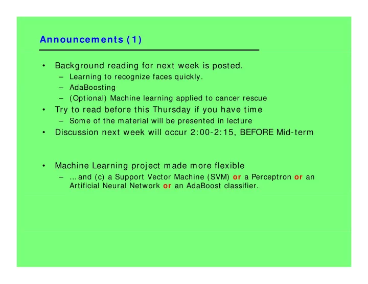
Announcem ents ( 1 ) • Background reading for next week is posted. – Learning to recognize faces quickly. – AdaBoosting AdaBoosting – (Optional) Machine learning applied to cancer rescue • Try to read before this Thursday if you have time – Some of the material will be presented in lecture p • Discussion next week will occur 2: 00-2: 15, BEFORE Mid-term • Machine Learning project made more flexible – … and (c) a Support Vector Machine (SVM) or a Perceptron or an Artificial Neural Network or an AdaBoost classifier.
Announcem ents ( 2 ) Hello, I have posted my changes at: http: / / code.google.com/ p/ maze- solver-game/ g I think there may be also be bug in the isVisible() function that checks if an edge can be drawn between two points for certain edge cases. (I haven't done much testing so I can't say definitively). definitively). As I find and fix bugs, I'll continue posting them, and others in the class email me their Gmail address, I can give them committing access as well. Similarly, if you have Google account, I can add you as a project owner if you send me your username you as a project owner, if you send me your username. A bit of a side note... The project is stored in a Mercurial repository. Mercurial can be downloaded from: http: / / mercurial.selenic.com/ A good tutorial by Joel Spolsky (Joel on Software): http: / / hginit.com/ --David
I ntoduction to Machine Learning i Reading for today: 18.1-18.4 L hi M t ti d t I
Outline • Different types of learning problems • • Different types of learning algorithms Different types of learning algorithms • Supervised learning – Decision trees Decision trees – Naïve Bayes – Perceptrons, Multi-layer Neural Networks – Boosting • Unsupervised Learning – K-means • Applications: learning to detect faces in images • Reading for today’s lecture: Chapter 18.1 to 18.4 (inclusive)
Autom ated Learning • Why is it useful for our agent to be able to learn? – Learning is a key hallmark of intelligence – The ability of an agent to take in real data and feedback and improve performance over time • Types of learning yp g – Supervised learning • Learning a mapping from a set of inputs to a target variable – Classification: target variable is discrete (e.g., spam email) – Regression: target variable is real-valued (e g stock market) Regression: target variable is real valued (e.g., stock market) – Unsupervised learning • No target variable provided – Clustering: grouping data into K groups Clustering: grouping data into K groups – Other types of learning • Reinforcement learning: e.g., game-playing agent • L Learning to rank, e.g., document ranking in Web search i t k d t ki i W b h • And many others… .
Sim ple illustrative learning problem Problem: decide whether to wait for a table at a restaurant, based on the following attributes: 1 1. Alternate: is there an alternative restaurant nearby? Alternate: is there an alternative restaurant nearby? 2. Bar: is there a comfortable bar area to wait in? 3. Fri/ Sat: is today Friday or Saturday? 4. Hungry: are we hungry? 5. 5 Patrons: number of people in the restaurant (None Some Full) Patrons: number of people in the restaurant (None, Some, Full) 6. Price: price range ($, $$, $$$) 7. Raining: is it raining outside? 8. Reservation: have we made a reservation? 9. 9. Type: kind of restaurant (French, Italian, Thai, Burger) Type: kind of restaurant (French, Italian, Thai, Burger) 10. WaitEstimate: estimated waiting time (0-10, 10-30, 30-60, > 60)
Training Data for Supervised Learning
Term inology • Attributes – Also known as features, variables, independent variables, covariates co a a es • Target Variable – Also known as goal predicate, dependent variable, … • Classification – Also known as discrimination, supervised classification, … • Error function – Objective function loss function Objective function, loss function, …
I nductive learning • Let x represent the input vector of attributes • • Let f(x) represent the value of the target variable for x Let f(x) represent the value of the target variable for x – The implicit mapping from x to f(x) is unknown to us – We just have training data pairs, D = { x, f(x)} available • We want to learn a mapping from x to f, i.e., h(x; ) is “close” to f(x) for all training data points x are the parameters of our predictor h(..) • • Examples: Examples: h(x; ) = sign(w 1 x 1 + w 2 x 2 + w 3 ) – – h k (x) = (x1 OR x2) AND (x3 OR NOT(x4)) k ( ) ( ) ( ( ))
Em pirical Error Functions • Empirical error function: E(h) = x distance[ h(x; ) , f] e.g., distance = squared error if h and f are real-valued (regression) distance = delta-function if h and f are categorical (classification) Sum is over all training pairs in the training data D S i ll t i i i i th t i i d t D In learning, we get to choose 1. what class of functions h(..) that we want to learn – potentially a huge space! (“hypothesis space”) potentially a huge space! ( hypothesis space ) 2. what error function/ distance to use - should be chosen to reflect real “loss” in problem - but often chosen for mathematical/ algorithmic convenience b f h f h i l/ l i h i i
I nductive Learning as Optim ization or Search • Empirical error function: E(h) = x distance[ h(x; ) , f] Empirical learning = finding h(x), or h(x; ) that minimizes E(h) • – In simple problems there may be a closed form solution • E.g., “normal equations” when h is a linear function of x, E = squared error – If E(h) is differentiable as a function of q, then we have a continuous optimization problem and can use gradient descent, etc • E.g., multi-layer neural networks – If E(h) is non-differentiable (e.g., classification), then we typically have a systematic search problem through the space of functions h problem through the space of functions h • E.g., decision tree classifiers • Once we decide on what the functional form of h is, and what the error function E is, then machine learning typically reduces to a large search or optimization i th hi l i t i ll d t l h ti i ti problem • Additional aspect: we really want to learn an h(..) that will generalize well to new data, not just memorize training data – will return to this later , j g
Our training data exam ple ( again) • If all attributes were binary, h(..) could be any arbitrary Boolean function • Natural error function E(h) to use is classification error, i.e., how many incorrect predictions does a hypothesis h make predictions does a hypothesis h make • Note an implicit assumption: – For any set of attribute values there is a unique target value – This in effect assumes a “no-noise” mapping from inputs to targets pp g p g • This is often not true in practice (e.g., in medicine). Will return to this later
Learning Boolean Functions • Given examples of the function, can we learn the function? • How many Boolean functions can be defined on d attributes? How many Boolean functions can be defined on d attributes? – Boolean function = Truth table + column for target function (binary) Truth table has 2 d rows – So there are 2 to the power of 2 d different Boolean functions we can define – (!) (!) – This is the size of our hypothesis space – E.g., d = 6, there are 18.4 x 10 18 possible Boolean functions • Observations: – Huge hypothesis spaces –> directly searching over all functions is impossible – Given a small data (n pairs) our learning problem may be underconstrained • Ockham’s razor: if multiple candidate functions all explain the data equally well, pick the simplest explanation (least complex function) • Constrain our search to classes of Boolean functions, e.g., – decision trees – Weighted linear sums of inputs (e.g., perceptrons)
Constrain h(..) to be a decision tree Decision Tree Learning •
Decision Tree Representations • Decision trees are fully expressive – can represent any Boolean function – Every path in the tree could represent 1 row in the truth table – Yi ld Yields an exponentially large tree ti ll l t Truth table is of size 2 d , where d is the number of attributes •
Decision Tree Representations • Trees can be very inefficient for certain types of functions – Parity function: 1 only if an even number of 1’s in the input vector • Trees are very inefficient at representing such functions – Majority function: 1 if more than ½ the inputs are 1’s • Also inefficient – Simple DNF formulae can be easily represented • E E.g., f = (A AND B) OR (NOT(A) AND D) f (A AND B) OR (NOT(A) AND D) • DNF = disjunction of conjunctions • Decision trees are in effect DNF representations – often used in practice since they often result in compact approximate f f representations for complex functions – E.g., consider a truth table where most of the variables are irrelevant to the function
Recommend
More recommend
Explore More Topics
Stay informed with curated content and fresh updates.
