and Economic Growth: Evidences from Time Series Data of Bangladesh - PowerPoint PPT Presentation

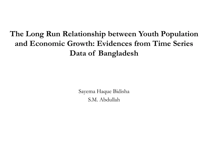
The Long Run Relationship between Youth Population and Economic Growth: Evidences from Time Series Data of Bangladesh Sayema Haque Bidisha S.M. Abdullah

Background • The composition of population and its rule in growth and development prospects • Contribution to labor market, in particular, the proportional size as well as the trend of youth population is of vital importance. • From Global point of view: the world now hosts ever largest young people: aged between 10 to 24 and in many countries of the world, the proportion of youth to the population is also showing a rising trend (UNFPA, 2014) Positive outcome Raise in as Growth the Improvem proportion ent of working Increase in age Youth Population Population

Background Contd. • Context of Bangladesh (LFS, 2013): Within the age group of 15 to 29 years, there was around 43.4 million people. • Youth population consisted of around 28 percent of total population of the country. • This rise in youth population has been reflected in the trend of youth labor force Year Youth Labor Force (15 – 29 Years), Source: LFS, 2013 2002 - 03 19 Million 2013 23.4 Million • This increased youth labor force if coupled with essential education and skill then it could turn into a vital factor for Bangladesh economy. • Against this backdrop, this paper utilized time series data of Bangladesh and attempted to understand the long run effect of proportional increase in youth population of the growth of gross domestic product of the country.

Review of Existing Literatures Paper Data and Methodology and Findings Area/Countrty Estimation Thuku et Time Series Data, VAR Model Positive relationship between population al. (2013) Kenya growth and economic growth Roudi Middle East and Descriptive and Proper balance between social safety net (2011) North Africa Graphical Analysis programs and market mechanisms to utilize youth population Iqbal Time Series (1974 ARDL Bound Testing Positive and significant impact of (2015) – 2011), Pakistan and Cointegration working age population on economic Approach growth Nakibullah Time Series (1959 VAR Model and For Bangladesh Per Capita Real GDP (1998) – 90), Bangladesh Granger Causality Granger cause population growth but reverse causality was not found to be valid. Population growth thus can be treated as endogenous. Ali et al. Time Series (1981 Simple Growth Model, Negative impact of Population Growth (2015) – 2014), OLS on Economic Development Bangladesh Ashford Sub – Saharan Comparative Analysis Emphasized on Schooling, Prevention (2007) Africa and Projections of Early Marriage, Family Planning Programs to reap the benefits of increased youth population

Data and Methodology • Purpose: Estimating the long run impact of proportional increase in youth population on the Growth of GDP • Data Duration: Time Series – 1972 to 2014, (WDI, World Bank) • A simple growth model with human capital as well as physical capital being the key factors of growth has been estimated. Variable Description GDPG Growth of Real GDP GDPSPSE GDP share of public spending on education SGER Secondary gross enrolment rate GDPSGFCF GDP share of gross fixed capital formation GDPSTRADE GDP share of trade RYP Proportion of youths in total population

Data and Methodology Contd. • Identification of Integration Order of the Variables: In particular, the following test regression has been estimated for each of the variables for testing the stationarity following Augmented Dickey Fuller (ADF) test procedure : • Selection of Lag Length: Selection of suitable lag length is important because introducing too many lags is argued to waste degrees of freedom, while too few lags might lead to the problem of misspecfication and is likely to cause autocorrelation in the residuals. Here, the appropriate lag length was selected using a multivariate version of BIC and AIC.

Data and Methodology Contd. • Johansen Cointegration Test (Johansen, 1988): Widely used for the presence of multiple cointegrating vectors and for the speed of adjustment parameter. It relies on the relationship between rank of a matrix and its characteristic roots. Consider the following generalization: • It can be expressed in difference form as follows: • By allowing for higher order auto regressive process the above model can be written as: • In the above process we will be focusing on the estimate of autoregressive coefficient and its corresponding characteristics roots. For performing the test following two test statistics is used:

Summary Statistics of the Key Variables Table 1: Summary Statistics of Key Variables GDPG RYP Correlation (P – Value) Year Mean Std. Deviation Mean Std. Deviation 1972 – 80 1.764 7.070 23.388 0.437 -0.477(0.193) 1981 – 90 4.021 1.549 26.984 1.453 -0.292(0.411) 1991 – 2000 4.680 0.624 29.024 0.139 0.443(0.198) 0.708 * (0.021) 2001 – 10 5.578 0.994 29.472 0.129 2011 – 14 6.265 0.264 28.977 0.169 0.840(0.160) 0.336 * (0.027) 1972 - 2014 4.273 3.538 27.469 2.423 Note: * indicates 5 percent level of significance • During early years average GDPG was low with a high standard deviation. The correlation among GDPG and RYP found to be negative and insignificant when sub samples has been considered. • Average GDPG was increasing along with its consistency and the correlation coefficient turned out to become positive during 1990s. • When the overall sample has been considered the correlation among these two variables has been found to be positive and significant. • Thus, our descriptive statistics therefore provides evidence of plausible positive impact of proportional increase in youth population in economic growth for Bangladesh- the impact of change in RYP on GDPG could be considered as a long run phenomena for Bangladesh.

Estimation Results: Stationarity Check Table A1: ADF Test for Checking Stationarity ADF Test Results, Null Hypothesis: Series Contains a Unit Root None Constant Constant and Trend Test Variables Test Stationari Stationari Test Stationari P Statisti P P Statistic ty ty Statistic ty c Non Non -12.837 * GDPG 0.458 0.80 -1.038 0.72 0.00 Stationary Stationary Stationary Stationarit Stationarit -3.809 * -3.786 * -3.644 ** D(GDPG) 0.00 0.00 0.03 Stationary y: I(1) y: I(1) Non Non Non GDPSPSE -0.59 0.45 -0.993 0.74 -0.98 0.93 Stationary Stationary Stationary D(GDPSPS Stationarit Stationarit Stationarit -5.453 * -5.418 * -5.381 * 0.00 0.00 0.00 E) y: I(1) y: I(1) y: I(1) Non Non Non SGER 1.789 0.98 0.244 0.97 -2.972 0.15 Stationary Stationary Stationary Stationarit Stationarit Stationarit -2.991 * -3.587 * -3.787 ** D(SGER) 0.00 0.01 0.02 y: I(1) y: I(1) y: I(1) Non Non Non GDPSGFCF 4.336 1.00 -1.333 0.60 -2.378 0.38 Stationary Stationary Stationary D(GDPSGF Stationarit Stationarit Stationarit -3.370 * -4.697 * -4.727 * 0.00 0.00 0.00 CF) y: I(1) y: I(1) y: I(1) GDPSTRA Non Non Non 0.941 0.90 -0.504 0.88 -2.454 0.34 DE Stationary Stationary Stationary D(GDPSTR Stationarit Stationarit Stationarit -7.186 * -7.544 * -7.636 * 0.00 0.00 0.00 ADE) y: I(1) y: I(1) y: I(1) Non Non -3.704 * RYP 0.767 0.87 0.00 Stationary -1.419 0.83 Stationary Stationary Stationarit Non Stationarit -1.720 *** D(RYP) 0.08 -1.995 0.28 -5.590* 0.00 y: I(1) Stationary y: I(1) Note: * indicates one percent level of significance, ** indicates five percent level of significance and *** indicates ten percent level of significance.

Lag Selection Table A2: VAR Lag Structure Selection Lag AIC BIC Endogenous Variables: GDPG, RYP, GDPSGFCF, GDPSPSE, GDPSTRADE, SGER 0 24.009 24.265 1 11.239 13.031 2 9.072 12.399* 3 8.670 13.533 4 6.980* 13.379 Note: * Indicates Lag Order selected by the respective criterion

Johansen Cointegration Test Hypothesized No. of CE(s) Eigenvalue Trace Statistic 0.05 Critical Value Prob.** Unrestricted Cointegration Rank Test (Trace) None* 0.6722 147.419 95.753 0.000 At most 1* 0.6114 102.800 69.818 0.000 At most 2* 0.5445 64.986 47.856 0.000 At most 3* 0.4001 33.525 29.797 0.017 At most 4 0.2640 13.083 15.494 0.111 Trace test indicates 4 cointegrating eqn(s) at the 0.05 level, * denotes rejection of the hypothesis at the 0.05 level, **MacKinnon-Haug-Michelis (1999) p-values Hypothesized No. of CE(s) Eigenvalue Max - Eigen Statistic 0.05 Critical Value Prob.** Unrestricted Cointegration Rank Test (Maximum Eigenvalue) None * 0.6722 44.618 40.077 0.014 At most 1* 0.6114 37.814 33.876 0.016 At most 2* 0.5445 31.460 27.584 0.015 At most 3 0.4001 20.441 21.131 0.062 At most 4 0.2640 12.261 14.264 0.101 Max-eigenvalue test indicates 3 cointegrating eqn(s) at the 0.05 level, * denotes rejection of the hypothesis at the 0.05 level, **MacKinnon-Haug-Michelis (1999) p-values