Analysis of tandem fluid queues Magorzata OReilly 1 Werner - PowerPoint PPT Presentation
Model and preliminaries Analysis and numerics Analysis of tandem fluid queues Magorzata OReilly 1 Werner Scheinhardt 2 1 Discipline of Mathematics, University of Tasmania 2 Department of Applied Mathematics, University of Twente MAM 2016
Model and preliminaries Analysis and numerics Analysis of tandem fluid queues Małgorzata O’Reilly 1 Werner Scheinhardt 2 1 Discipline of Mathematics, University of Tasmania 2 Department of Applied Mathematics, University of Twente MAM 2016 1/33 Małgorzata O’Reilly, Werner Scheinhardt Analysis of tandem fluid queues
Model and preliminaries Analysis and numerics Outline Model and preliminaries 1 Analysis and numerics 2 2/33 Małgorzata O’Reilly, Werner Scheinhardt Analysis of tandem fluid queues
Model and preliminaries Analysis and numerics Outline Model and preliminaries 1 Analysis and numerics 2 3/33 Małgorzata O’Reilly, Werner Scheinhardt Analysis of tandem fluid queues
Model and preliminaries Analysis and numerics Model: two fluid queues driven by ϕ ( t ) CTMC ϕ ( t ) with finite state space S , generator T Two fluid queues, contents X ( t ) and Y ( t ) , both ∈ [ 0 , ∞ ) 4/33 Małgorzata O’Reilly, Werner Scheinhardt Analysis of tandem fluid queues
Model and preliminaries Analysis and numerics First queue X ( t ) driven by ϕ ( t ) ( ϕ ( t ) , X ( t )) is standard fluid queue Fluid rates in R = diag ( r i ) i ∈S d dt X ( t ) = r ϕ ( t ) when X ( t ) > 0 , d dt X ( t ) = max ( 0 , r ϕ ( t ) ) when X ( t ) = 0 . S = S + ∪ S − ∪ S � , e.g. S + = { i ∈ S : r i > 0 } (upstates, downstates, zero-states) also: S ⊖ = S − ∪ S � (“zero-states at X ( t ) = 0”) after ordering, T ++ T + − T + � . T = T − + T −− T − � T � + T � − T �� 5/33 Małgorzata O’Reilly, Werner Scheinhardt Analysis of tandem fluid queues
Model and preliminaries Analysis and numerics Second queue Y ( t ) driven by ( ϕ ( t ) , X ( t )) � Y ( t ) increases when X ( t ) > 0, at rate � c i > 0 Y ( t ) decreases when X ( t ) = 0, at rate c i < 0 (unless Y ( t ) = 0) So � d dt Y ( t ) = � c ϕ ( t ) > 0 when X ( t ) > 0 , d dt Y ( t ) = c ϕ ( t ) < 0 when X ( t ) = 0 , Y ( t ) > 0 , � d � dt Y ( t ) = � c ϕ ( t ) · 1 { ϕ ( t ) ∈ S + } when X ( t ) = 0 , Y ( t ) = 0 . � C = diag ( � c i ) i ∈S and C = diag ( c i ) i ∈S 6/33 Małgorzata O’Reilly, Werner Scheinhardt Analysis of tandem fluid queues
� C i <0 ^ r i <0 r i >0 C i >0 Model and preliminaries Analysis and numerics � Special case: S � = ∅ , |S + | = |S − | = 1 , C = − C = I Y(t) X(t) t Y(t) v t X(t) [Kroese and Scheinhardt. Joint Distributions for Interacting Fluid Queues, Queueing Systems , 2001] 7/33 Małgorzata O’Reilly, Werner Scheinhardt Analysis of tandem fluid queues
r i >0 r i <0 C i >0 ^ C i <0 Model and preliminaries Analysis and numerics Qualitative behaviour Y(t) X(t) t Y(t) v t X(t) Assuming stability (see paper) process ( ϕ ( t ) , X ( t ) , Y ( t )) alternates between: (i) periods on x = 0 (ii) periods on x > 0 8/33 Małgorzata O’Reilly, Werner Scheinhardt Analysis of tandem fluid queues
r i >0 r i <0 C i >0 ^ C i <0 Model and preliminaries Analysis and numerics Qualitative behaviour (i) on x = 0 Y(t) X(t) t Y(t) v t X(t) (i) periods on x = 0 Y ( t ) decreasing, unless at x = 0 , y = 0 ϕ ( t ) in S ⊖ starts at x = 0 , y > 0, with ϕ ( t ) in S − ends at x = 0 , y ≥ 0, with ϕ ( t ) jumping from S ⊖ to S + 9/33 Małgorzata O’Reilly, Werner Scheinhardt Analysis of tandem fluid queues
r i >0 r i <0 C i >0 ^ C i <0 Model and preliminaries Analysis and numerics Qualitative behaviour (ii) on x > 0 Y(t) X(t) t Y(t) v t X(t) (ii) periods on x > 0 Y ( t ) increasing (while X ( t ) can either increase or decrease) ϕ ( t ) in S (any phase) starts at x = 0 , y ≥ 0, with ϕ ( t ) ∈ S + ends at x = 0 , y > 0, with ϕ ( t ) ∈ S − 10/33 Małgorzata O’Reilly, Werner Scheinhardt Analysis of tandem fluid queues
Model and preliminaries Analysis and numerics Stationary distribution has following form (all vectors with |S| components): (i) 1-dimensional densities π ( 0 , y ) at x = 0 , y > 0 point masses p ( 0 , 0 ) at ( 0 , 0 ) (ii) 2-dimensional densities π ( x , y ) on { ( x , y ) : x > 0 , y > x · min i ∈S + { � c i / r i }} 1-dimensional density π i ( x , x � c i / r i ) on line y = x � c i / r i , i ∈ S + 11/33 Małgorzata O’Reilly, Werner Scheinhardt Analysis of tandem fluid queues
Model and preliminaries Analysis and numerics Outline Model and preliminaries 1 Analysis and numerics 2 12/33 Małgorzata O’Reilly, Werner Scheinhardt Analysis of tandem fluid queues
Model and preliminaries Analysis and numerics Approach Several steps: Introduce embedded discrete-time process J k Find its stationary distribution ξ y Take a deep breath... Express π ( 0 , y ) and p ( 0 , 0 ) in ξ y , using down-shift in Y Normalise based on knowledge of ( ϕ ( t ) , X ( t )) Express π ( x , y ) in π ( 0 , y ) and p ( 0 , 0 ) , using up-shift in Y Express π i ( x , x � c i / r i ) in p ( 0 , 0 ) Mostly as LST’s (but not always) 13/33 Małgorzata O’Reilly, Werner Scheinhardt Analysis of tandem fluid queues
Model and preliminaries Analysis and numerics Approach Several steps: Introduce embedded discrete-time process J k Find its stationary distribution ξ y Take a deep breath... Express π ( 0 , y ) and p ( 0 , 0 ) in ξ y , using down-shift in Y Normalise based on knowledge of ( ϕ ( t ) , X ( t )) Express π ( x , y ) in π ( 0 , y ) and p ( 0 , 0 ) , using up-shift in Y Express π i ( x , x � c i / r i ) in p ( 0 , 0 ) Mostly as LST’s (but not always) 13/33 Małgorzata O’Reilly, Werner Scheinhardt Analysis of tandem fluid queues
Model and preliminaries Analysis and numerics Approach Several steps: Introduce embedded discrete-time process J k Find its stationary distribution ξ y Take a deep breath... Express π ( 0 , y ) and p ( 0 , 0 ) in ξ y , using down-shift in Y Normalise based on knowledge of ( ϕ ( t ) , X ( t )) Express π ( x , y ) in π ( 0 , y ) and p ( 0 , 0 ) , using up-shift in Y Express π i ( x , x � c i / r i ) in p ( 0 , 0 ) Mostly as LST’s (but not always) 13/33 Małgorzata O’Reilly, Werner Scheinhardt Analysis of tandem fluid queues
� � Model and preliminaries Analysis and numerics Intermezzo (i) on down-shift: Q ⊖⊖ and Q ⊖ + � � Define generator matrix C ⊖ | ) − 1 T ⊖⊖ , Q ⊖⊖ = ( | then for i , j ∈ S ⊖ , and z > 0 , � Q ⊖⊖ z ] ij = P ( ϕ ( t z ) = j , ϕ ( u ) ∈ S ⊖ , 0 ≤ u ≤ t z | ϕ ( 0 ) = i , X ( 0 ) = 0 ) � � [ e Also, C ⊖ | ) − 1 T ⊖ + , Q ⊖ + = ( | is a matrix of transition rates (w.r.t. level) to phases in S + (for times at which X and Y start increasing) [Bean, O’Reilly and Taylor. Hitting probabilities and hitting times for stochastic fluid flows, SPA 2005] 14/33 Małgorzata O’Reilly, Werner Scheinhardt Analysis of tandem fluid queues
Model and preliminaries Analysis and numerics Intermezzo (ii) on up-shift: � Q ( s ) and � Ψ ( s ) � t Let θ = inf { t > 0 : X ( t ) = 0 } and U ( t ) = u = 0 � c ϕ ( u ) du , then U ( θ ) is total up-shift in Y during Busy Period of X Its |S + | × |S − | density matrix � ψ ( z ) is given via LST � ∞ e − sz � � Ψ ( s ) = ψ ( z ) dz , z = 0 as [ � Ψ ( s )] ij = E ( e − sU ( θ ) 1 { ϕ ( θ ) = j } | ϕ ( 0 ) = i , X ( 0 ) = 0 ) , [Bean and O’Reilly. A stochastic two-dimensional fluid model, Stochastic Models , 2013] 15/33 Małgorzata O’Reilly, Werner Scheinhardt Analysis of tandem fluid queues
Model and preliminaries Analysis and numerics Intermezzo (ii) on up-shift: � Q ( s ) and � Ψ ( s ) To find � Ψ ( s ) define Key generator matrix � Q ( s ) , as � � � � Q ( s ) ++ Q ( s ) + − � Q ( s ) = � � Q ( s ) − + Q ( s ) −− Q ( s ) ++ = ( R + ) − 1 � � � T ++ − s � C + − T + � ( T �� − s � C � ) − 1 T � + Q ( s ) + − = ( R + ) − 1 � � � T + − − T + � ( T �� − s � C � ) − 1 T � − Q ( s ) − + = ( | R − | ) − 1 � � � T − + − T − � ( T �� − s � C � ) − 1 T � + Q ( s ) −− = ( | R − | ) − 1 � � � T −− − s � C − − T − � ( T �� − s � C � ) − 1 T � − Then � Ψ ( s ) is minimum nonnegative solution of Riccati eq. Q ( s ) + − + � � Ψ ( s ) � Ψ ( s ) � Q ( s ) ++ � Ψ ( s ) + � Q ( s ) −− + � Q ( s ) − + � Ψ ( s ) = O , [Bean and O’Reilly. A stochastic two-dimensional fluid model, Stochastic Models , 2013] 16/33 Małgorzata O’Reilly, Werner Scheinhardt Analysis of tandem fluid queues
Model and preliminaries Analysis and numerics Back on track... Embedded process J k Let J k = ( ϕ ( θ k ) , Y ( θ k )) , with state space S − × ( 0 , ∞ ) , where θ k is k -th time that ( ϕ ( t ) , X ( t ) , Y ( t )) hits x = 0 Lemma � The transition kernel of J k is given by � � z � � � � Q ⊖ + � Q ⊖⊖ u P z , y = I O e ψ ( y − z + u ) du � u =[ z − y ] + � � Q ⊖ + � Q ⊖⊖ z ( − Q ⊖⊖ ) − 1 + I O e ψ ( y ) . � � where [ x ] + denotes max ( 0 , x ) , and I O is a |S − | × |S ⊖ | matrix. 17/33 Małgorzata O’Reilly, Werner Scheinhardt Analysis of tandem fluid queues
Recommend
More recommend
Explore More Topics
Stay informed with curated content and fresh updates.
