
An Incremental Algorithm for Computing Cylindrical Algebraic - PowerPoint PPT Presentation
An Incremental Algorithm for Computing Cylindrical Algebraic Decompositions Changbo Chen, Marc Moreno Maza ORCCA, University of Western Ontario, Canada Oct. 27, 2012 ASCM 2012, Beijing, China Cylindrical Algebraic Decomposition (CAD) of R n A
An Incremental Algorithm for Computing Cylindrical Algebraic Decompositions Changbo Chen, Marc Moreno Maza ORCCA, University of Western Ontario, Canada Oct. 27, 2012 ASCM 2012, Beijing, China
Cylindrical Algebraic Decomposition (CAD) of R n A CAD of R n is a partition of R n such that each cell in the partition is a connected semi-algebraic subset of R n and all the cells are cylindrically arranged. Two subsets A and B of R n are called cylindrically arranged if for any 1 ≤ k ≤ n , the projections of A and B on R k are either equal or disjoint.
Cylindrical algebraic decomposition (CAD) Invented by G.E. Collins in 1973 for solving Real Quantifier Elimination (QE) problems. Previous work on CAD Adjacency and clustering techniques (D. Arnon, G.E. Collins and S. McCallum 84), Improved projection operator (H. Hong 90; S. McCallum 88, 98; C. Brown 01), Partially built CAD s (Collins and Hong 91, A. Strzebo´ nski 00), Improved stack construction (G.E. Collins, J.R. Johnson, and W. Krandick), Efficient projection orders (A. Dolzmann, A. Seidl and T. Sturm 04), Making use of equational constraints (G.E. Collins 98; C. Brown and S. McCallum 05), Computing CAD via triangular decompositions (C. Chen, M. Moreno Maza, B. Xia and L. Yang 09), Preprocessing input by Gr¨ obner bases (B. Buchberger and H. Hong 91; D.J. Wilson, R.J. Bradford, and J.H. Davenport 12), Set-theoretical operations by CAD (A. Strzebo´ nski 10) · · · Software Qepcad , Mathematica, Redlog, SyNRAC, TCAD (Since Maple 14).
Outline 1 First Idea: Introduce Case Discussion 2 Second Idea: Compute the Decomposition Incrementally 3 Third Idea: Compute CAD of a Variety 4 Implementation and Benchmark
Outline 1 First Idea: Introduce Case Discussion 2 Second Idea: Compute the Decomposition Incrementally 3 Third Idea: Compute CAD of a Variety 4 Implementation and Benchmark
CAD based on projection-lifting scheme (PCAD) Projection Let Proj be a projection operator. Repeatedly apply Proj : Proj Proj Proj F n ( x 1 , . . . , x n ) − − − → F n − 1 ( x 1 , . . . , x n − 1 ) − − − → · · · − − − → F 1 ( x 1 ) . Lifting The real roots of the polynomials in F 1 plus the open intervals between them form an F 1 -invariant CAD of R 1 . For each cell C of the F k − 1 invariant CAD of R k − 1 , isolate the polynomials of F k at a sample point of C , which produces all the cells of the F k -invariant CAD of R k above C .
CAD based on triangular decompositions (TCAD) Motivation: potential drawback of Collins’ scheme The projection operator is a function defined independently of the input system. As a result, a strong projection operator (Collins-Hong operator) usually produces much more polynomials than needed. A weak projection operator (McCalumn-Brown operator) may fail for non-generic cases. Solution: make case discussion during projection Case discussion is common for algorithms computing triangular decomposition. At ISSAC’09, we (with B. Xia and L. Yang) introduced case discussion (as in triangular decomposition of polynomials systems) into CAD computation. As a result, the projection phase in classical CAD algorithm is replaced by computing a complex cylindrical tree.
Complex cylindrical tree let α = ( α 1 , . . . , α n − 1 ) ∈ C n − 1 define C [ x 1 , . . . , x n ] Φ α − − → C [ x n ] , where p ( x 1 , . . . , x n ) �→ p ( α, x n ) Separation Let S ⊂ C n − 1 and P ⊂ k [ x 1 , . . . , x n − 1 , x n ] be a finite set of level n polynomials. We say that P separates above S if for each α ∈ S : for each p ∈ P , Φ α (leading coefficient of p w . r . t . x n ) � = 0 for all p ∈ P , Φ α ( p ) are squarefree and coprime. A { y 2 + x, y 2 + y } -sign invariant complex cylindrical tree x 2 + x � = 0 x + 1 = 0 x = 0 y 2 + x = 0 ( y 2 + x )( y 2 + y ) � = 0 y = 0 y + 1 = 0 y − 1 = 0 y 2 + y � = 0 y 3 − y � = 0 y 2 + y = 0 y = 0 y + 1 = 0
Rethink classical CAD in terms of complex cylindrical tree The projection factors are a, b, c, 4 ac − b 2 , ax 2 + bx + c . c = 0 any x b = 0 c � = 0 any x ax 2 + bx + c = 0 a = 0 c = 0 ax 2 + bx + c � = 0 b � = 0 ax 2 + bx + c = 0 c � = 0 ax 2 + bx + c � = 0 ax 2 + bx + c = 0 4 ac − b 2 = 0 ax 2 + bx + c � = 0 b = 0 ax 2 + bx + c = 0 4 ac − b 2 � = 0 ax 2 + bx + c � = 0 ax 2 + bx + c = 0 a � = 0 c = 0 ax 2 + bx + c � = 0 ax 2 + bx + c = 0 4 ac − b 2 = 0 b � = 0 ax 2 + bx + c � = 0 ax 2 + bx + c = 0 c (4 ac − b 2 ) � = 0 ax 2 + bx + c � = 0
The complex cylindrical tree constructed by TCAD any x c = 0 b = 0 c � = 0 any x a = 0 bx + c = 0 b � = 0 any c bx + c � = 0 2 ax + b = 0 4 ac − b 2 = 0 2 ax + b � = 0 a � = 0 any b ax 2 + bx + c = 0 4 ac − b 2 � = 0 ax 2 + bx + c � = 0
Outline 1 First Idea: Introduce Case Discussion 2 Second Idea: Compute the Decomposition Incrementally 3 Third Idea: Compute CAD of a Variety 4 Implementation and Benchmark
The refinement operation Input A y 2 + x sign invariant complex cylindrical tree � y = 0 y 2 + x = 0 : x = 0 y 2 + x � = 0 y � = 0 : T := � y 2 + x = 0 y 2 + x = 0 : x � = 0 y 2 + x � = 0 y 2 + x � = 0 : A polynomial y 2 + y . Output The tree T is refined into a new one, above each path of which both y 2 + x and y 2 + y are sign invariant.
Refine the first path of the tree with y 2 + y � y = 0 y 2 + x = 0 : x = 0 y 2 + x � = 0 y � = 0 : x � = 0 · · · � y = 0 y 2 + x = 0 ∧ y 2 + y = 0 : x = 0 y 2 + x � = 0 y � = 0 : ⇒ x � = 0 · · ·
Refine the next path of the tree with y 2 + y � y = 0 y 2 + x = 0 ∧ y 2 + y = 0 : x = 0 y 2 + x � = 0 y � = 0 : x � = 0 · · · y 2 + x = 0 ∧ y 2 + y = 0 y = 0 : y 2 + x � = 0 ∧ y 2 + y = 0 x = 0 y = − 1 : y 2 + x � = 0 ∧ y 2 + y � = 0 ⇒ otherwise : x � = 0 · · ·
The { y 2 + x, y 2 + y } sign invariant cylindrical tree of C 2 y 2 + x = 0 ∧ y 2 + y = 0 y = 0 : y 2 + x � = 0 ∧ y 2 + y = 0 x = 0 y = − 1 : y 2 + x � = 0 ∧ y 2 + y � = 0 otherwise : y 2 + x = 0 ∧ y 2 + y = 0 y = − 1 : y 2 + x = 0 ∧ y 2 + y � = 0 y = 1 : x = − 1 y 2 + x � = 0 ∧ y 2 + y = 0 y = 0 : y 2 + x � = 0 ∧ y 2 + y � = 0 otherwise : y 2 + x = 0 y 2 + x = 0 ∧ y 2 + y � = 0 : y 2 + y = 0 y 2 + x � = 0 ∧ y 2 + y = 0 otherwise : y 2 + x � = 0 ∧ y 2 + y � = 0 otherwise :
x = 0 x � = 0 y 2 + x = 0 y 2 + x � = 0 y = 0 y � = 0 x 2 + x � = 0 x + 1 = 0 x = 0 y 2 + x = 0 ( y 2 + x )( y 2 + y ) � = 0 y = 0 y + 1 = 0 y − 1 = 0 y = 0 y 2 + y � = 0 y 3 − y � = 0 y 2 + y = 0 y + 1 = 0
Outline 1 First Idea: Introduce Case Discussion 2 Second Idea: Compute the Decomposition Incrementally 3 Third Idea: Compute CAD of a Variety 4 Implementation and Benchmark
Compute partial cylindrical tree A partial cylindrical tree induced by the F := { y 2 + x = 0 , y 2 + y = 0 } is x = 0 x + 1 = 0 y = 0 y + 1 = 0
Transform a complex cylindrical decomposition to a real one y 2 + x = 0 � y = 0 : x = 0 y 2 + x � = 0 y � = 0 : Complex : y 2 + x = 0 y 2 + x = 0 � : x � = 0 y 2 + x � = 0 y 2 + x � = 0 : y 2 + x > 0 � y < − | x | : y 2 + x = 0 � y = − | x | : y 2 + x < 0 � � x < 0 y > − | x | ∧ y < | x | : y 2 + x = 0 � y = | x | : y 2 + x > 0 � y > | x | : Real : y 2 + x > 0 y < 0 : y 2 + x = 0 x = 0 y = 0 : y 2 + x > 0 y > 0 : for any y : y 2 + x > 0 x > 0
Outline 1 First Idea: Introduce Case Discussion 2 Second Idea: Compute the Decomposition Incrementally 3 Third Idea: Compute CAD of a Variety 4 Implementation and Benchmark
Implementation in Maple The universe tree is always up-to-date 0 0 0 Split Deep Copy 8 2 7 1 2 2 7 8 3 4 5 6 3 4 5 6 9 10 11 12 5 6 A sub-tree evolves with the universe tree 0 0 0 1 7 8 7 8 4 4 4 10 12
tcd-rec : our ISSAC’09 recursive algorithm tcd-inc : the incremental algorithm
tcd-inc: the incremental algorithm with set of polynomials as input tcd-eqs: the incremental algorithm with set of equations as input
Conclusion and work in progress Conclusion We presented an incremental algorithm for computing CADs. The core operation of our algorithm is an Intersect operation, which refines a complex cylindrical tree with a polynomial constraint. The Intersect operation provides an systematic solution for propagating equational constraints. For many examples, the incremental outperforms both Qepcad and Mathematica as well as our previous recursive algorithms. Work in progress We have developed a preliminary QE routine Qetcad based on TCAD. We are working on different optimizations for both Tcad and Qetcad .
Recommend


More recommend
Explore More Topics
Stay informed with curated content and fresh updates.